Décomposition d’une série temporelle
Ce notebook présente quelques étapes simples pour une série temporelle. La plupart utilise le module statsmodels.tsa.
Données
Les données sont artificielles mais simulent ce que pourraient être le chiffre d’affaires d’un magasin de quartier, des samedi très forts, une semaine morne, un Noël chargé, un été plat.
[10]:
import pandas
from teachpyx.datasets.data_ts import generate_sells

df = pandas.DataFrame(generate_sells())
df.head()
[10]:
| date | value | |
|---|---|---|
| 0 | 2023-03-06 00:39:51.820916 | 0.005036 |
| 1 | 2023-03-07 00:39:51.820916 | 0.004769 |
| 2 | 2023-03-08 00:39:51.820916 | 0.006293 |
| 3 | 2023-03-09 00:39:51.820916 | 0.006932 |
| 4 | 2023-03-10 00:39:51.820916 | 0.008666 |
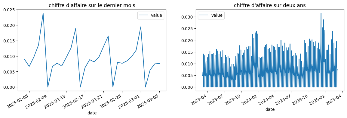
Premiers graphiques
La série a deux saisonnalités, hebdomadaire, mensuelle.
[11]:
import matplotlib.pyplot as plt

fig, ax = plt.subplots(1, 2, figsize=(14, 4))
df.iloc[-30:].set_index("date").plot(ax=ax[0])
df.set_index("date").plot(ax=ax[1])
ax[0].set_title("chiffre d'affaire sur le dernier mois")
ax[1].set_title("chiffre d'affaire sur deux ans")
[11]:
Text(0.5, 1.0, "chiffre d'affaire sur deux ans")
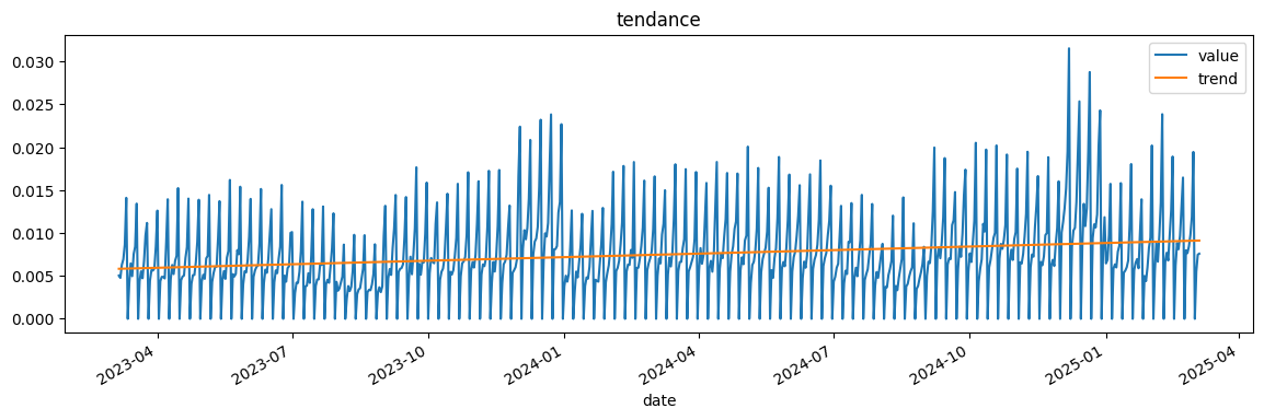
Elle a une vague tendance, on peut calculer un tendance à l’ordre 1, 2, …
[12]:
from statsmodels.tsa.tsatools import detrend

notrend = detrend(df.value, order=1)
df["notrend"] = notrend
df["trend"] = df["value"] - notrend
ax = df.plot(x="date", y=["value", "trend"], figsize=(14, 4))
ax.set_title("tendance")
[12]:
Text(0.5, 1.0, 'tendance')
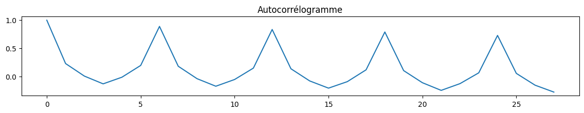
Autocorrélations…
[13]:
from statsmodels.tsa.stattools import acf

cor = acf(df.value)
cor
[13]:
array([ 1.00000000e+00,  2.05522806e-02, -5.81441890e-02, -2.01231811e-02,
       -2.50535358e-02, -6.81166704e-02,  5.94423981e-04,  9.25077506e-01,
       -3.79860291e-03, -8.24593539e-02, -4.47874626e-02, -4.84700550e-02,
       -9.04852284e-02, -2.10021533e-02,  8.86200829e-01, -2.87651649e-02,
       -1.01244603e-01, -6.63494241e-02, -6.78568361e-02, -1.06899756e-01,
       -3.87558669e-02,  8.53901943e-01, -4.51168979e-02, -1.16356930e-01,
       -8.69970753e-02, -8.95201510e-02, -1.25409915e-01, -6.73383807e-02,
        8.10734998e-01])
[14]:
fig, ax = plt.subplots(1, 1, figsize=(14, 2))
ax.plot(cor)
ax.set_title("Autocorrélogramme")
[14]:
Text(0.5, 1.0, 'Autocorrélogramme')
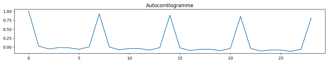
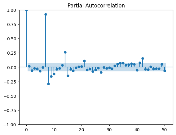
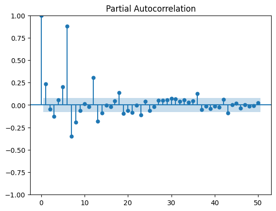
La première saisonalité apparaît, 7, 14, 21… Les autocorrélations partielles confirment cela, plutôt 7 jours.
[15]:
from statsmodels.tsa.stattools import pacf
from statsmodels.graphics.tsaplots import plot_pacf

plot_pacf(df.value, lags=50)
[15]:

Comme il n’y a rien le dimanche, il vaut mieux les enlever. Garder des zéros nous priverait de modèles multiplicatifs.
[16]:
df["weekday"] = df.date.dt.weekday
df.head()
[16]:
| date | value | notrend | trend | weekday | |
|---|---|---|---|---|---|
| 0 | 2023-03-06 00:39:51.820916 | 0.005036 | -0.000797 | 0.005833 | 0 |
| 1 | 2023-03-07 00:39:51.820916 | 0.004769 | -0.001068 | 0.005837 | 1 |
| 2 | 2023-03-08 00:39:51.820916 | 0.006293 | 0.000451 | 0.005842 | 2 |
| 3 | 2023-03-09 00:39:51.820916 | 0.006932 | 0.001086 | 0.005846 | 3 |
| 4 | 2023-03-10 00:39:51.820916 | 0.008666 | 0.002815 | 0.005851 | 4 |
[17]:
df_nosunday = df[df.weekday != 6]
df_nosunday.head(n=10)
[17]:
| date | value | notrend | trend | weekday | |
|---|---|---|---|---|---|
| 0 | 2023-03-06 00:39:51.820916 | 0.005036 | -0.000797 | 0.005833 | 0 |
| 1 | 2023-03-07 00:39:51.820916 | 0.004769 | -0.001068 | 0.005837 | 1 |
| 2 | 2023-03-08 00:39:51.820916 | 0.006293 | 0.000451 | 0.005842 | 2 |
| 3 | 2023-03-09 00:39:51.820916 | 0.006932 | 0.001086 | 0.005846 | 3 |
| 4 | 2023-03-10 00:39:51.820916 | 0.008666 | 0.002815 | 0.005851 | 4 |
| 5 | 2023-03-11 00:39:51.820916 | 0.014102 | 0.008247 | 0.005855 | 5 |
| 7 | 2023-03-13 00:39:51.820916 | 0.004139 | -0.001725 | 0.005864 | 0 |
| 8 | 2023-03-14 00:39:51.820916 | 0.006453 | 0.000584 | 0.005869 | 1 |
| 9 | 2023-03-15 00:39:51.820916 | 0.004974 | -0.000900 | 0.005873 | 2 |
| 10 | 2023-03-16 00:39:51.820916 | 0.007552 | 0.001674 | 0.005878 | 3 |
[18]:
fig, ax = plt.subplots(1, 1, figsize=(14, 2))
cor = acf(df_nosunday.value)
ax.plot(cor)
ax.set_title("Autocorrélogramme");
[19]:
plot_pacf(df_nosunday.value, lags=50);
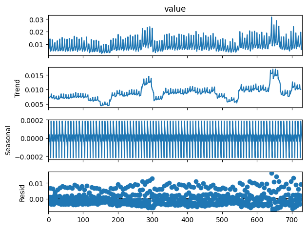
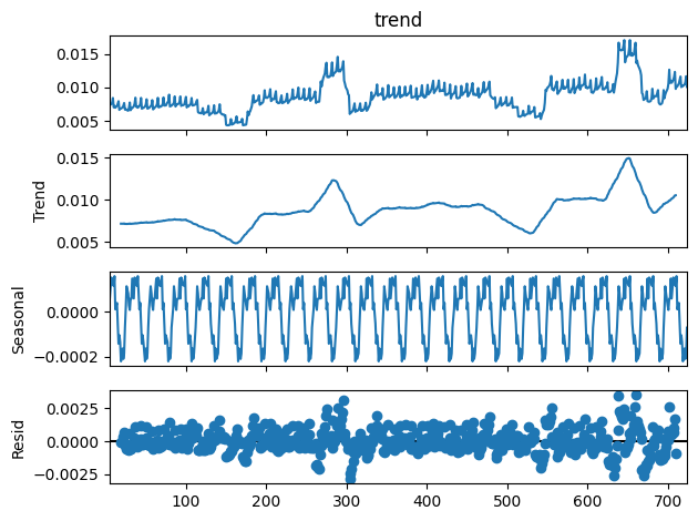
On décompose la série en tendance + saisonnalité. Les étés et Noël apparaissent.
[21]:
from statsmodels.tsa.seasonal import seasonal_decompose

res = seasonal_decompose(df_nosunday.value, period=7)
res.plot();
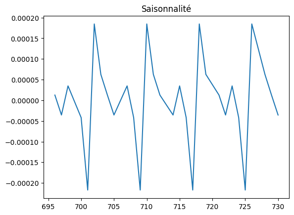
[22]:
plt.plot(res.seasonal[-30:])
plt.title("Saisonnalité")
[22]:
Text(0.5, 1.0, 'Saisonnalité')
[24]:
cor = acf(res.trend[5:-5], fft=True)
plt.plot(cor)
[24]:
[<matplotlib.lines.Line2D at 0x7f0cd93f1d30>]
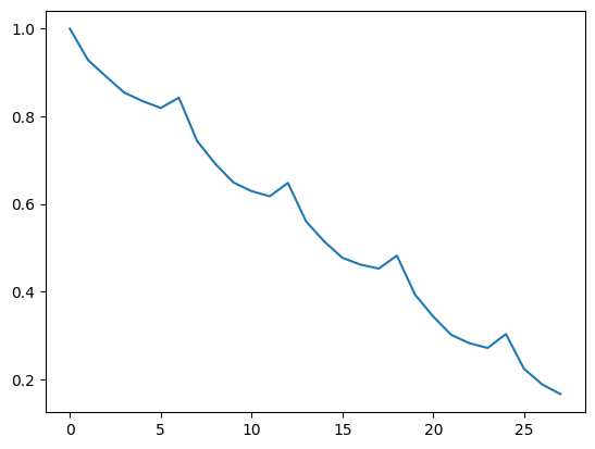
On cherche maintenant la saisonnalité de la série débarrassée de sa tendance herbdomadaire. On retrouve la saisonnalité mensuelle.
[25]:
res_year = seasonal_decompose(res.trend[5:-5], period=25)
res_year.plot()
[25]:

Test de stationnarité
Le test KPSS permet de tester la stationnarité d’une série.
[26]:
from statsmodels.tsa.stattools import kpss

kpss(res.trend[5:-5])
/tmp/ipykernel_59627/406539216.py:2: InterpolationWarning: The test statistic is outside of the range of p-values available in the
look-up table. The actual p-value is smaller than the p-value returned.

  kpss(res.trend[5:-5])
[26]:
(np.float64(1.245031416161398),
 np.float64(0.01),
 16,
 {'10%': 0.347, '5%': 0.463, '2.5%': 0.574, '1%': 0.739})
Comme ce n’est pas toujours facile à interpréter, on simule une variable aléatoire gaussienne donc sans tendance.
[27]:
from numpy.random import randn

bruit = randn(1000)
kpss(bruit)
/tmp/ipykernel_59627/3765297593.py:3: InterpolationWarning: The test statistic is outside of the range of p-values available in the
look-up table. The actual p-value is greater than the p-value returned.

  kpss(bruit)
[27]:
(np.float64(0.11384797070848017),
 np.float64(0.1),
 1,
 {'10%': 0.347, '5%': 0.463, '2.5%': 0.574, '1%': 0.739})
Et puis une série avec une tendance forte.
[28]:
from numpy.random import randn
from numpy import arange

bruit = randn(1000) * 100 + arange(1000) / 10
kpss(bruit)
/tmp/ipykernel_59627/2615492180.py:4: InterpolationWarning: The test statistic is outside of the range of p-values available in the
look-up table. The actual p-value is smaller than the p-value returned.

  kpss(bruit)
[28]:
(np.float64(4.201503723150045),
 np.float64(0.01),
 11,
 {'10%': 0.347, '5%': 0.463, '2.5%': 0.574, '1%': 0.739})
Une valeur forte indique une tendance et la série en a clairement une.
Prédiction
Les modèles AR, ARMA, ARIMA se concentrent sur une série à une dimension. En machine learning, il y a la série et plein d’autres informations. On construit une matrice avec des séries décalées.
[29]:
from statsmodels.tsa.tsatools import lagmat

lag = 8
X = lagmat(df_nosunday["value"], lag)
lagged = df_nosunday.copy()
for c in range(1, lag + 1):
    lagged["lag%d" % c] = X[:, c - 1]
lagged.tail()
[29]:
| date | value | notrend | trend | weekday | lag1 | lag2 | lag3 | lag4 | lag5 | lag6 | lag7 | lag8 | |
|---|---|---|---|---|---|---|---|---|---|---|---|---|---|
| 725 | 2025-02-28 00:39:51.820916 | 0.011877 | 0.002777 | 0.009100 | 4 | 0.009749 | 0.008428 | 0.007654 | 0.007989 | 0.016468 | 0.013102 | 0.009676 | 0.008109 |
| 726 | 2025-03-01 00:39:51.820916 | 0.019454 | 0.010350 | 0.009105 | 5 | 0.011877 | 0.009749 | 0.008428 | 0.007654 | 0.007989 | 0.016468 | 0.013102 | 0.009676 |
| 728 | 2025-03-03 00:39:51.820916 | 0.005494 | -0.003620 | 0.009114 | 0 | 0.019454 | 0.011877 | 0.009749 | 0.008428 | 0.007654 | 0.007989 | 0.016468 | 0.013102 |
| 729 | 2025-03-04 00:39:51.820916 | 0.007479 | -0.001639 | 0.009118 | 1 | 0.005494 | 0.019454 | 0.011877 | 0.009749 | 0.008428 | 0.007654 | 0.007989 | 0.016468 |
| 730 | 2025-03-05 00:39:51.820916 | 0.007589 | -0.001534 | 0.009123 | 2 | 0.007479 | 0.005494 | 0.019454 | 0.011877 | 0.009749 | 0.008428 | 0.007654 | 0.007989 |
On ajoute ou on réécrit le jour de la semaine qu’on utilise comme variable supplémentaire.
[30]:
lagged["weekday"] = lagged.date.dt.weekday
[31]:
X = lagged.drop(["date", "value", "notrend", "trend"], axis=1)
Y = lagged["value"]
X.shape, Y.shape
[31]:
((627, 9), (627,))
[32]:
from numpy import corrcoef

corrcoef(X)
~/vv/this312/lib/python3.12/site-packages/numpy/lib/_function_base_impl.py:3045: RuntimeWarning: invalid value encountered in divide
  c /= stddev[:, None]
~/vv/this312/lib/python3.12/site-packages/numpy/lib/_function_base_impl.py:3046: RuntimeWarning: invalid value encountered in divide
  c /= stddev[None, :]
[32]:
array([[        nan,         nan,         nan, ...,         nan,
                nan,         nan],
       [        nan,  1.        ,  0.99999247, ..., -0.69791204,
         0.99986414,  0.99996236],
       [        nan,  0.99999247,  1.        , ..., -0.69925528,
         0.99991238,  0.99996712],
       ...,
       [        nan, -0.69791204, -0.69925528, ...,  1.        ,
        -0.70192748, -0.70219418],
       [        nan,  0.99986414,  0.99991238, ..., -0.70192748,
         1.        ,  0.99987949],
       [        nan,  0.99996236,  0.99996712, ..., -0.70219418,
         0.99987949,  1.        ]], shape=(627, 627))
Etrange autant de grandes valeurs, cela veut dire que la tendance est trop forte pour calculer des corrélations, il vaudrait mieux tout recommencer avec la série  . Bref, passons…
[33]:
X.columns
[33]:
Index(['weekday', 'lag1', 'lag2', 'lag3', 'lag4', 'lag5', 'lag6', 'lag7',
       'lag8'],
      dtype='object')
Une régression linéaire car les modèles linéaires sont toujours de bonnes baseline et pour connaître le modèle simulé, on ne fera pas beaucoup mieux.
[34]:
from sklearn.linear_model import LinearRegression

clr = LinearRegression()
clr.fit(X, Y)
[34]:
LinearRegression()In a Jupyter environment, please rerun this cell to show the HTML representation or trust the notebook.
On GitHub, the HTML representation is unable to render, please try loading this page with nbviewer.org.
LinearRegression()
[35]:
from sklearn.metrics import r2_score

r2_score(Y, clr.predict(X))
[35]:
0.8750652931937053
[36]:
clr.coef_
[36]:
array([ 0.00171654,  0.35489858,  0.2667268 ,  0.07460985,  0.01104078,
       -0.06234941,  0.37933643, -0.12027835, -0.05625968])
On retrouve la saisonnalité,  et
et  sont de mèches.
[37]:
for i in range(1, X.shape[1]):
    print("X(t-%d)" % (i), r2_score(Y, X.iloc[:, i]))
X(t-1) -0.5343370770216411
X(t-2) -0.9776153682766282
X(t-3) -1.2540090159405772
X(t-4) -1.01367860631983
X(t-5) -0.602451646171541
X(t-6) 0.7635187615860253
X(t-7) -0.6454355106118854
X(t-8) -1.0867844309933337
Auparavant (l’année dernière en fait), je construisais deux bases, apprentissage et tests, comme ceci :
[38]:
n = X.shape[0]
X_train = X.iloc[: n * 2 // 3]
X_test = X.iloc[n * 2 // 3 :]
Y_train = Y[: n * 2 // 3]
Y_test = Y[n * 2 // 3 :]
Et puis scikit-learn est arrivée avec TimeSeriesSplit.
[39]:
from sklearn.model_selection import TimeSeriesSplit

tscv = TimeSeriesSplit(n_splits=5)
for train_index, test_index in tscv.split(lagged):
    data_train, data_test = lagged.iloc[train_index, :], lagged.iloc[test_index, :]
    print("TRAIN:", data_train.shape, "TEST:", data_test.shape)
TRAIN: (107, 13) TEST: (104, 13)
TRAIN: (211, 13) TEST: (104, 13)
TRAIN: (315, 13) TEST: (104, 13)
TRAIN: (419, 13) TEST: (104, 13)
TRAIN: (523, 13) TEST: (104, 13)
Et on calé une forêt aléatoire…
[40]:
import warnings
from sklearn.ensemble import RandomForestRegressor

clr = RandomForestRegressor()


def train_test(clr, train_index, test_index):
    data_train = lagged.iloc[train_index, :]
    data_test = lagged.iloc[test_index, :]
    clr.fit(
        data_train.drop(["value", "date", "notrend", "trend"], axis=1), data_train.value
    )
    r2 = r2_score(
        data_test.value,
        clr.predict(
            data_test.drop(["value", "date", "notrend", "trend"], axis=1).values
        ),
    )
    return r2


warnings.simplefilter("ignore")
last_test_index = None
for train_index, test_index in tscv.split(lagged):
    r2 = train_test(clr, train_index, test_index)
    if last_test_index is not None:
        r2_prime = train_test(clr, last_test_index, test_index)
        print(r2, r2_prime)
    else:
        print(r2)
    last_test_index = test_index
0.7830797306279333
0.7892143392871785 0.710251489079545
0.926515934247996 0.9254337080628354
0.811090703869577 0.7717494202307796
0.7646201099598264 0.6571969210691542
2 ans coupé en 5, soit tous les 5 mois, ça veut dire que ce découpage inclut parfois Noël, parfois l’été et que les performances y seront très sensibles.
[41]:
from sklearn.metrics import r2_score

r2 = r2_score(
    data_test.value,
    clr.predict(data_test.drop(["value", "date", "notrend", "trend"], axis=1).values),
)
r2
[41]:
0.6571969210691542
On compare avec le  avec le même obtenu en utilisant
  ,
,  , …
, …  comme prédiction.
[42]:
for i in range(1, 9):
    print(i, ":", r2_score(data_test.value, data_test["lag%d" % i]))
1 : -0.5315727068325993
2 : -1.0250735581487076
3 : -1.3208901364676007
4 : -1.074139284130378
5 : -0.6238251202278204
6 : 0.657764576444329
7 : -0.7208207891388771
8 : -1.1824818758877917
[43]:
lagged[:5]
[43]:
| date | value | notrend | trend | weekday | lag1 | lag2 | lag3 | lag4 | lag5 | lag6 | lag7 | lag8 | |
|---|---|---|---|---|---|---|---|---|---|---|---|---|---|
| 0 | 2023-03-06 00:39:51.820916 | 0.005036 | -0.000797 | 0.005833 | 0 | 0.000000 | 0.000000 | 0.000000 | 0.000000 | 0.0 | 0.0 | 0.0 | 0.0 |
| 1 | 2023-03-07 00:39:51.820916 | 0.004769 | -0.001068 | 0.005837 | 1 | 0.005036 | 0.000000 | 0.000000 | 0.000000 | 0.0 | 0.0 | 0.0 | 0.0 |
| 2 | 2023-03-08 00:39:51.820916 | 0.006293 | 0.000451 | 0.005842 | 2 | 0.004769 | 0.005036 | 0.000000 | 0.000000 | 0.0 | 0.0 | 0.0 | 0.0 |
| 3 | 2023-03-09 00:39:51.820916 | 0.006932 | 0.001086 | 0.005846 | 3 | 0.006293 | 0.004769 | 0.005036 | 0.000000 | 0.0 | 0.0 | 0.0 | 0.0 |
| 4 | 2023-03-10 00:39:51.820916 | 0.008666 | 0.002815 | 0.005851 | 4 | 0.006932 | 0.006293 | 0.004769 | 0.005036 | 0.0 | 0.0 | 0.0 | 0.0 |
En fait le jour de la semaine est une variable catégorielle, on crée une colonne par jour.
[44]:
from sklearn.compose import ColumnTransformer
from sklearn.preprocessing import OneHotEncoder
[45]:
cols = ["lag1", "lag2", "lag3", "lag4", "lag5", "lag6", "lag7", "lag8"]
ct = ColumnTransformer(
    [("pass", "passthrough", cols), ("dummies", OneHotEncoder(), ["weekday"])]
)
pred = ct.fit(lagged).transform(lagged[:5])
pred
[45]:
array([[0.        , 0.        , 0.        , 0.        , 0.        ,
        0.        , 0.        , 0.        , 1.        , 0.        ,
        0.        , 0.        , 0.        , 0.        ],
       [0.00503561, 0.        , 0.        , 0.        , 0.        ,
        0.        , 0.        , 0.        , 0.        , 1.        ,
        0.        , 0.        , 0.        , 0.        ],
       [0.00476948, 0.00503561, 0.        , 0.        , 0.        ,
        0.        , 0.        , 0.        , 0.        , 0.        ,
        1.        , 0.        , 0.        , 0.        ],
       [0.00629279, 0.00476948, 0.00503561, 0.        , 0.        ,
        0.        , 0.        , 0.        , 0.        , 0.        ,
        0.        , 1.        , 0.        , 0.        ],
       [0.00693242, 0.00629279, 0.00476948, 0.00503561, 0.        ,
        0.        , 0.        , 0.        , 0.        , 0.        ,
        0.        , 0.        , 1.        , 0.        ]])
On met tout dans un pipeline parce que c’est plus joli, plus pratique aussi.
[46]:
from sklearn.pipeline import make_pipeline
from sklearn.decomposition import PCA, TruncatedSVD

cols = ["lag1", "lag2", "lag3", "lag4", "lag5", "lag6", "lag7", "lag8"]
model = make_pipeline(
    make_pipeline(
        ColumnTransformer(
            [
                ("pass", "passthrough", cols),
                (
                    "dummies",
                    make_pipeline(OneHotEncoder(), TruncatedSVD(n_components=2)),
                    ["weekday"],
                ),
            ]
        ),
        LinearRegression(),
    )
)
model.fit(lagged, lagged["value"])
[46]:
Pipeline(steps=[('pipeline',
                 Pipeline(steps=[('columntransformer',
                                  ColumnTransformer(transformers=[('pass',
                                                                   'passthrough',
                                                                   ['lag1',
                                                                    'lag2',
                                                                    'lag3',
                                                                    'lag4',
                                                                    'lag5',
                                                                    'lag6',
                                                                    'lag7',
                                                                    'lag8']),
                                                                  ('dummies',
                                                                   Pipeline(steps=[('onehotencoder',
                                                                                    OneHotEncoder()),
                                                                                   ('truncatedsvd',
                                                                                    TruncatedSVD())]),
                                                                   ['weekday'])])),
                                 ('linearregression', LinearRegression())]))])
In a Jupyter environment, please rerun this cell to show the HTML representation or trust the notebook. On GitHub, the HTML representation is unable to render, please try loading this page with nbviewer.org.
Pipeline(steps=[('pipeline',
                 Pipeline(steps=[('columntransformer',
                                  ColumnTransformer(transformers=[('pass',
                                                                   'passthrough',
                                                                   ['lag1',
                                                                    'lag2',
                                                                    'lag3',
                                                                    'lag4',
                                                                    'lag5',
                                                                    'lag6',
                                                                    'lag7',
                                                                    'lag8']),
                                                                  ('dummies',
                                                                   Pipeline(steps=[('onehotencoder',
                                                                                    OneHotEncoder()),
                                                                                   ('truncatedsvd',
                                                                                    TruncatedSVD())]),
                                                                   ['weekday'])])),
('linearregression', LinearRegression())]))])Pipeline(steps=[('columntransformer',
ColumnTransformer(transformers=[('pass', 'passthrough',
                                 ['lag1', 'lag2', 'lag3', 'lag4', 'lag5',
                                  'lag6', 'lag7', 'lag8']),
                                ('dummies',
                                 Pipeline(steps=[('onehotencoder',
                                                  OneHotEncoder()),
                                                 ('truncatedsvd',
                                                  TruncatedSVD())]),
['weekday'])])),
('linearregression', LinearRegression())])ColumnTransformer(transformers=[('pass', 'passthrough',
['lag1', 'lag2', 'lag3', 'lag4', 'lag5',
'lag6', 'lag7', 'lag8']),
('dummies',
Pipeline(steps=[('onehotencoder',
OneHotEncoder()),
('truncatedsvd',
TruncatedSVD())]),
['weekday'])])['lag1', 'lag2', 'lag3', 'lag4', 'lag5', 'lag6', 'lag7', 'lag8']
passthrough
['weekday']
OneHotEncoder()
TruncatedSVD()
LinearRegression()
C’est plus facile à voir visuellement.
[47]:
r2_score(lagged["value"], model.predict(lagged))
[47]:
0.8302843587445363