Pivot de gauss avec numpy

Etape par étape, le pivote de Gauss implémenté en python puis avec numpy.

%matplotlib inline

Python

import numpy

def pivot_gauss(m):
    n = m.copy()
    for i in range(1, m.shape[0]):
        j0 = i
        while j0 < m.shape[0] and m[j0, i - 1] == 0:
            j0 += 1
        for j in range(j0, m.shape[0]):
            coef = -m[j, i - 1] / m[i - 1, i - 1]
            for k in range(i - 1, m.shape[1]):
                m[j, k] += coef * m[i - 1, k]
    return m


m = numpy.random.rand(4, 4)
piv = pivot_gauss(m)
piv * (numpy.abs(piv) > 1e-10)

array([[ 0.58650968,  0.72315516,  0.9137217 ,  0.04526746],
       [ 0.        ,  0.70012278,  0.87604076,  0.92402115],
       [ 0.        ,  0.        , -0.36865515,  1.00362559],
       [ 0.        ,  0.        ,  0.        ,  0.26361505]])

* (numpy.abs(piv) > 1e-10) sert à simplifier l’affichage des valeurs quasi nulles.

Numpy 1

def pivot_gauss2(m):
    n = m.copy()
    for i in range(1, m.shape[0]):
        j0 = i
        while j0 < m.shape[0] and m[j0, i - 1] == 0:
            j0 += 1
        for j in range(j0, m.shape[0]):
            coef = -m[j, i - 1] / m[i - 1, i - 1]
            m[j, i - 1 :] += m[i - 1, i - 1 :] * coef
    return m


piv = pivot_gauss2(m)
piv * (numpy.abs(piv) > 1e-10)

array([[ 0.58650968,  0.72315516,  0.9137217 ,  0.04526746],
       [ 0.        ,  0.70012278,  0.87604076,  0.92402115],
       [ 0.        ,  0.        , -0.36865515,  1.00362559],
       [ 0.        ,  0.        ,  0.        ,  0.26361505]])

Numpy 2

def pivot_gauss3(m):
    n = m.copy()
    for i in range(1, m.shape[0]):
        j0 = i
        while j0 < m.shape[0] and m[j0, i - 1] == 0:
            j0 += 1
        coef = -m[j0:, i - 1] / m[i - 1, i - 1]
        m[j0:, i - 1 :] += coef.reshape((-1, 1)) * m[i - 1, i - 1 :].reshape((1, -1))
    return m


piv = pivot_gauss3(m)
piv * (numpy.abs(piv) > 1e-10)

array([[ 0.58650968,  0.72315516,  0.9137217 ,  0.04526746],
       [ 0.        ,  0.70012278,  0.87604076,  0.92402115],
       [ 0.        ,  0.        , -0.36865515,  1.00362559],
       [ 0.        ,  0.        ,  0.        ,  0.26361505]])

Vitesse

from tqdm import tqdm
import pandas
from teachpyx.ext_test_case import measure_time

data = []
for n in tqdm([10, 20, 30, 40, 50, 60, 70, 80, 100]):
    m = numpy.random.rand(n, n)
    if n < 50:
        res = measure_time(lambda: pivot_gauss(m), number=10, repeat=10)
        res.update(dict(name="python", n=n))
        data.append(res)
    res = measure_time(lambda: pivot_gauss2(m), number=10, repeat=10)
    res.update(dict(name="numpy1", n=n))
    data.append(res)
    res = measure_time(lambda: pivot_gauss3(m), number=10, repeat=10)
    res.update(dict(name="numpy2", n=n))
    data.append(res)

df = pandas.DataFrame(data)
df

100%|██████████| 9/9 [00:07<00:00,  1.17it/s]

	average	deviation	min_exec	max_exec	repeat	number	ttime	context_size	warmup_time	name	n
0	0.000051	0.000030	0.000028	0.000125	10	10	0.000512	64	0.000728	python	10
1	0.000045	0.000021	0.000028	0.000094	10	10	0.000447	64	0.000046	numpy1	10
2	0.000137	0.000024	0.000110	0.000197	10	10	0.001367	64	0.000253	numpy2	10
3	0.001134	0.000540	0.000623	0.002258	10	10	0.011340	64	0.003184	python	20
4	0.001312	0.000678	0.000639	0.002858	10	10	0.013121	64	0.001035	numpy1	20
5	0.000375	0.000184	0.000233	0.000818	10	10	0.003753	64	0.001292	numpy2	20
6	0.001557	0.001094	0.000686	0.003803	10	10	0.015571	64	0.016613	python	30
7	0.000404	0.000062	0.000331	0.000553	10	10	0.004045	64	0.000364	numpy1	30
8	0.000471	0.000037	0.000440	0.000545	10	10	0.004713	64	0.000482	numpy2	30
9	0.003798	0.001491	0.002594	0.007715	10	10	0.037978	64	0.018972	python	40
10	0.001324	0.000265	0.001054	0.002030	10	10	0.013239	64	0.001341	numpy1	40
11	0.000820	0.000190	0.000602	0.001140	10	10	0.008200	64	0.000651	numpy2	40
12	0.004260	0.001177	0.002724	0.006471	10	10	0.042603	64	0.005198	numpy1	50
13	0.001690	0.000268	0.001100	0.002116	10	10	0.016902	64	0.001080	numpy2	50
14	0.009320	0.002581	0.005762	0.013509	10	10	0.093197	64	0.015497	numpy1	60
15	0.001664	0.000133	0.001458	0.001827	10	10	0.016641	64	0.001309	numpy2	60
16	0.005314	0.001348	0.003848	0.008252	10	10	0.053141	64	0.016670	numpy1	70
17	0.001629	0.000216	0.001459	0.002045	10	10	0.016286	64	0.001499	numpy2	70
18	0.011036	0.003890	0.007070	0.018254	10	10	0.110356	64	0.017467	numpy1	80
19	0.002637	0.000582	0.001846	0.003606	10	10	0.026375	64	0.002417	numpy2	80
20	0.021563	0.003232	0.017314	0.029488	10	10	0.215629	64	0.028747	numpy1	100
21	0.004673	0.001109	0.003391	0.005935	10	10	0.046730	64	0.005792	numpy2	100

piv = df.pivot(index="n", columns="name", values="average")
piv

name	numpy1	numpy2	python
n
10	0.000045	0.000137	0.000051
20	0.001312	0.000375	0.001134
30	0.000404	0.000471	0.001557
40	0.001324	0.000820	0.003798
50	0.004260	0.001690	NaN
60	0.009320	0.001664	NaN
70	0.005314	0.001629	NaN
80	0.011036	0.002637	NaN
100	0.021563	0.004673	NaN

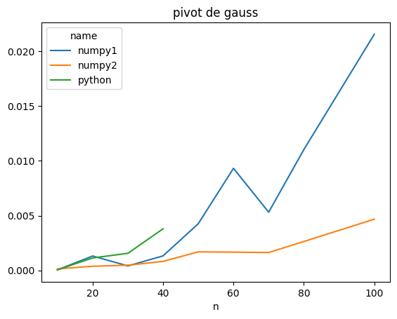
piv.plot(title="pivot de gauss");

---

Notebook on github