Régression polynômiale et pipeline#

Le notebook compare plusieurs de modèles de régression polynômiale.

[2]:

%matplotlib inline

[3]:

from teachpyx.datasets import load_wines_dataset

data = load_wines_dataset()
X = data.drop(["quality", "color"], axis=1)
y = data["quality"]

[4]:

from sklearn.model_selection import train_test_split

X_train, X_test, y_train, y_test = train_test_split(X, y)

On normalise les données. Pour ce cas particulier, c’est d’autant plus important que les polynômes prendront de très grandes valeurs si cela n’est pas fait et les librairies de calculs n’aiment pas les ordres de grandeurs trop différents.

[5]:

from sklearn.preprocessing import Normalizer

norm = Normalizer()
X_train_norm = norm.fit_transform(X_train)
X_test_norm = norm.transform(X_test)

La transformation PolynomialFeatures créée de nouvelles features en multipliant les variables les unes avec les autres. Pour le degré deux et trois features $a, b, c$ , on obtient les nouvelles features : $1, a, b, c, a^2, ab, ac, b^2, bc, c^2$ .

[6]:

from time import perf_counter
from sklearn.linear_model import LinearRegression
from sklearn.preprocessing import PolynomialFeatures
from sklearn.pipeline import make_pipeline
from sklearn.metrics import r2_score

r2ts = []
r2es = []
degs = []
tts = []
models = []

for d in range(1, 5):
    begin = perf_counter()
    pipe = make_pipeline(PolynomialFeatures(degree=d), LinearRegression())
    pipe.fit(X_train_norm, y_train)
    duree = perf_counter() - begin
    r2t = r2_score(y_train, pipe.predict(X_train_norm))
    r2e = r2_score(y_test, pipe.predict(X_test_norm))
    degs.append(d)
    r2ts.append(r2t)
    r2es.append(r2e)
    tts.append(duree)
    models.append(pipe)
    print(d, r2t, r2e, duree)

1 0.1909065078664849 0.16570749381482386 0.02195639999990817
2 0.31686272332465504 0.2634484656108902 0.16658860000006825
3 0.4117084105383497 -1.446755311176299 1.0382120000001578
4 0.5940872457783092 -3926.677572477097 2.8583189999999377

[7]:

import pandas

df = pandas.DataFrame(dict(temps=tts, r2_train=r2ts, r2_test=r2es, degré=degs))
df.set_index("degré")

[7]:

	temps	r2_train	r2_test
degré
1	0.021956	0.190907	0.165707
2	0.166589	0.316863	0.263448
3	1.038212	0.411708	-1.446755
4	2.858319	0.594087	-3926.677572

Le polynômes de degré 2 paraît le meilleur modèle. Le temps de calcul est multiplié par 10 à chaque fois, ce qui correspond au nombre de features. On voit néanmoins que l’ajout de features croisée fonctionne sur ce jeu de données. Mais au delà de 3, la régression produit des résultats très mauvais sur la base de test alors qu’ils continuent d’augmenter sur la base d’apprentissage. Voyons cela un peu plus en détail.

[7]:

import matplotlib.pyplot as plt

fig, ax = plt.subplots(1, 2, figsize=(12, 4))

n = 15
ax[0].plot(y_train[:n].reset_index(), "o")
ax[1].plot(y_test[:n].reset_index(), "o")
ax[0].set_title("Prédictions sur quelques valeurs\napprentissage")
ax[1].set_title("Prédictions sur quelques valeurs\ntest")
for x in ax:
    x.set_ylim([3, 9])
    x.get_xaxis().set_visible(False)

for model in models:
    d = model.get_params()["polynomialfeatures__degree"]
    tr = model.predict(X_train_norm[:n])
    te = model.predict(X_test_norm[:n])
    ax[0].plot(tr, label="d=%d" % d)
    ax[1].plot(te, label="d=%d" % d)
ax[0].legend()
ax[1].legend();

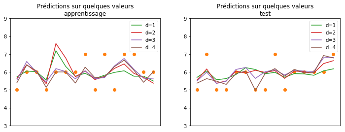
../../_images/practice_ml_winesr_reg_poly_10_0.png

Le modèle de degré 4 a l’air performant sur la base d’apprentissage mais s’égare complètement sur la base de test comme s’il était surpris des valeurs rencontrées sur la base de test. On dit que le modèle fait du sur-apprentissage ou overfitting en anglais. Le polynôme de degré fonctionne mieux que la régression linéaire simple. On peut se demander quelles sont les variables croisées qui ont un impact sur la performance. On utilise le modèle statsmodels.

[8]:

poly = PolynomialFeatures(degree=2)
poly_feat_train = poly.fit_transform(X_train_norm)
poly_feat_test = poly.fit_transform(X_test_norm)

[9]:

from statsmodels.regression.linear_model import OLS

model = OLS(y_train, poly_feat_train)
results = model.fit()
results.summary2()

[9]:

Model:	OLS	Adj. R-squared:	0.306
Dependent Variable:	quality	AIC:	10768.5223
Date:	2024-01-23 00:08	BIC:	11268.3493
No. Observations:	4872	Log-Likelihood:	-5307.3
Df Model:	76	F-statistic:	29.30
Df Residuals:	4795	Prob (F-statistic):	0.00
R-squared:	0.317	Scale:	0.52557

	Coef.	Std.Err.	t	P>\|t\|	[0.025	0.975]
const	874.2126	1866.6100	0.4683	0.6396	-2785.1996	4533.6248
x1	17.2438	25.1175	0.6865	0.4924	-31.9980	66.4856
x2	-735.9147	164.2593	-4.4802	0.0000	-1057.9383	-413.8911
x3	-375.2205	200.9788	-1.8670	0.0620	-769.2311	18.7900
x4	2.1457	13.7859	0.1556	0.8763	-24.8809	29.1723
x5	-1219.9140	760.0849	-1.6050	0.1086	-2710.0291	270.2011
x6	33.0684	8.6300	3.8318	0.0001	16.1496	49.9873
x7	45.6122	23.6785	1.9263	0.0541	-0.8085	92.0328
x8	-1621.7821	721.4602	-2.2479	0.0246	-3036.1752	-207.3890
x9	-123.6719	196.5043	-0.6294	0.5291	-508.9104	261.5667
x10	-213.6188	172.6441	-1.2373	0.2160	-552.0806	124.8429
x11	274.6811	25.3731	10.8257	0.0000	224.9381	324.4241
x12	-888.0924	1860.0506	-0.4775	0.6331	-4534.6449	2758.4602
x13	213.0448	149.3410	1.4266	0.1538	-79.7320	505.8216
x14	-169.2454	191.2389	-0.8850	0.3762	-544.1614	205.6706
x15	-2.3959	21.0911	-0.1136	0.9096	-43.7441	38.9523
x16	151.4367	661.2643	0.2290	0.8189	-1144.9447	1447.8180
x17	-13.3943	9.8122	-1.3651	0.1723	-32.6306	5.8421
x18	-12.3144	22.1599	-0.5557	0.5784	-55.7580	31.1291
x19	-228.1023	1055.2972	-0.2161	0.8289	-2296.9691	1840.7644
x20	263.5729	260.8085	1.0106	0.3123	-247.7314	774.8773
x21	210.1261	147.0152	1.4293	0.1530	-78.0912	498.3434
x22	-102.4573	26.1357	-3.9202	0.0001	-153.6952	-51.2193
x23	-1256.2263	1979.4050	-0.6346	0.5257	-5136.7684	2624.3158
x24	2503.6940	1629.0043	1.5369	0.1244	-689.9019	5697.2899
x25	-304.5840	139.4970	-2.1834	0.0291	-578.0621	-31.1060
x26	6503.3193	4276.6479	1.5207	0.1284	-1880.8729	14887.5116
x27	176.1465	65.4348	2.6919	0.0071	47.8643	304.4288
x28	541.9165	145.6814	3.7199	0.0002	256.3141	827.5190
x29	-5408.0462	5170.0682	-1.0460	0.2956	-15543.7521	4727.6598
x30	1591.6613	1576.5785	1.0096	0.3128	-1499.1559	4682.4786
x31	-3066.2318	1347.2069	-2.2760	0.0229	-5707.3755	-425.0882
x32	611.6934	183.2814	3.3375	0.0009	252.3778	971.0089
x33	861.9664	2070.4337	0.4163	0.6772	-3197.0336	4920.9664
x34	-307.3877	171.8498	-1.7887	0.0737	-644.2921	29.5168
x35	-8483.4913	6547.3948	-1.2957	0.1951	-21319.3893	4352.4067
x36	150.5489	83.1030	1.8116	0.0701	-12.3711	313.4689
x37	300.7497	178.4947	1.6849	0.0921	-49.1819	650.6813
x38	14067.7740	7800.2113	1.8035	0.0714	-1224.2191	29359.7672
x39	-5133.5558	2077.6861	-2.4708	0.0135	-9206.7738	-1060.3378
x40	-2372.2746	1576.8448	-1.5044	0.1325	-5463.6139	719.0647
x41	708.8006	236.3385	2.9991	0.0027	245.4687	1172.1325
x42	-910.1293	1867.0943	-0.4875	0.6260	-4570.4908	2750.2323
x43	1971.4865	757.4887	2.6027	0.0093	486.4611	3456.5118
x44	-7.6328	5.0273	-1.5183	0.1290	-17.4886	2.2230
x45	2.8665	12.6000	0.2275	0.8200	-21.8354	27.5684
x46	1429.2194	705.7754	2.0250	0.0429	45.5757	2812.8631
x47	-287.7160	203.0709	-1.4168	0.1566	-685.8281	110.3961
x48	-189.7045	168.1916	-1.1279	0.2594	-519.4371	140.0282
x49	-18.0129	19.5540	-0.9212	0.3570	-56.3477	20.3219
x50	10142.2002	7074.9790	1.4335	0.1518	-3728.0049	24012.4054
x51	-201.9536	331.1123	-0.6099	0.5419	-851.0857	447.1785
x52	1197.2260	682.4747	1.7542	0.0795	-140.7375	2535.1896
x53	20265.9335	23064.5613	0.8787	0.3796	-24951.1898	65483.0568
x54	-12226.8108	6517.5063	-1.8760	0.0607	-25004.1137	550.4920
x55	-3613.4768	4978.7999	-0.7258	0.4680	-13374.2092	6147.2555
x56	2196.0436	843.4185	2.6037	0.0092	542.5563	3849.5310
x57	-909.6884	1867.1743	-0.4872	0.6261	-4570.2067	2750.8299
x58	-24.9437	7.6926	-3.2426	0.0012	-40.0247	-9.8627
x59	549.2329	298.2374	1.8416	0.0656	-35.4492	1133.9150
x60	-13.8185	79.9507	-0.1728	0.8628	-170.5585	142.9216
x61	59.9612	69.6414	0.8610	0.3893	-76.5679	196.4903
x62	-60.9958	9.6344	-6.3310	0.0000	-79.8838	-42.1079
x63	-915.2771	1867.4927	-0.4901	0.6241	-4576.4197	2745.8655
x64	856.3795	643.6237	1.3306	0.1834	-405.4183	2118.1773
x65	172.8750	176.1471	0.9814	0.3264	-172.4541	518.2041
x66	233.8040	154.5694	1.5126	0.1304	-69.2230	536.8310
x67	-208.7613	22.8714	-9.1276	0.0000	-253.5998	-163.9229
x68	2377.5655	18554.7387	0.1281	0.8980	-33998.2360	38753.3671
x69	11008.3563	10291.6307	1.0696	0.2848	-9167.9622	31184.6748
x70	-6367.0944	6065.2219	-1.0498	0.2939	-18257.7123	5523.5234
x71	-2160.1700	944.6336	-2.2868	0.0223	-4012.0853	-308.2546
x72	-4031.2392	1137.0986	-3.5452	0.0004	-6260.4741	-1802.0043
x73	1604.8538	1639.6859	0.9788	0.3277	-1609.6830	4819.3905
x74	766.9861	249.3365	3.0761	0.0021	278.1721	1255.8001
x75	-2563.1016	2045.6050	-1.2530	0.2103	-6573.4261	1447.2228
x76	596.8511	210.7614	2.8319	0.0046	183.6620	1010.0402
x77	-1033.7653	1865.5885	-0.5541	0.5795	-4691.1748	2623.6442

Omnibus:	74.655	Durbin-Watson:	2.012
Prob(Omnibus):	0.000	Jarque-Bera (JB):	119.025
Skew:	0.141	Prob(JB):	0.000
Kurtosis:	3.712	Condition No.:	4390541685726112

Notes:
[1] Standard Errors assume that the covariance matrix of the errors is correctly specified.
[2] The smallest eigenvalue is 7.09e-28. This might indicate that there are strong multicollinearity problems or that the design matrix is singular.

Ce n’est pas très lisible. Il faut ajouter le nom de chaque variable et recommencer.

[12]:

names = poly.get_feature_names_out(input_features=data.columns[:-2])
names = [n.replace(" ", " * ") for n in names]
pft = pandas.DataFrame(poly_feat_train, columns=names)
pft.head()

[12]:

	1	fixed_acidity	volatile_acidity	citric_acid	residual_sugar	chlorides	free_sulfur_dioxide	total_sulfur_dioxide	density	pH	...	density^2	density * pH	density * sulphates	density * alcohol	pH^2	pH * sulphates	pH * alcohol	sulphates^2	sulphates * alcohol	alcohol^2
0	1.0	0.061316	0.003511	0.003461	0.019779	0.000455	0.306582	0.939526	0.009773	0.030263	...	0.000096	0.000296	0.000044	0.001315	0.000916	0.000138	0.004070	0.000021	0.000612	0.018090
1	1.0	0.035236	0.001373	0.001922	0.065438	0.000206	0.205924	0.974706	0.004572	0.014552	...	0.000021	0.000067	0.000013	0.000192	0.000212	0.000042	0.000613	0.000008	0.000121	0.001772
2	1.0	0.042579	0.001319	0.001919	0.101349	0.000336	0.293852	0.947522	0.005996	0.020210	...	0.000036	0.000121	0.000014	0.000345	0.000408	0.000046	0.001163	0.000005	0.000131	0.003314
3	1.0	0.053638	0.000920	0.001456	0.037547	0.000421	0.206890	0.973147	0.007627	0.025210	...	0.000058	0.000192	0.000024	0.000549	0.000636	0.000079	0.001816	0.000010	0.000226	0.005188
4	1.0	0.071498	0.002413	0.002949	0.010725	0.000447	0.366428	0.920540	0.008848	0.026812	...	0.000078	0.000237	0.000036	0.000981	0.000719	0.000108	0.002971	0.000016	0.000446	0.012282

5 rows × 78 columns

[13]:

results.summary2(xname=pft.columns)

[13]:

Model:	OLS	Adj. R-squared:	0.306
Dependent Variable:	quality	AIC:	10768.5223
Date:	2024-01-23 00:09	BIC:	11268.3493
No. Observations:	4872	Log-Likelihood:	-5307.3
Df Model:	76	F-statistic:	29.30
Df Residuals:	4795	Prob (F-statistic):	0.00
R-squared:	0.317	Scale:	0.52557

	Coef.	Std.Err.	t	P>\|t\|	[0.025	0.975]
1	874.2126	1866.6100	0.4683	0.6396	-2785.1996	4533.6248
fixed_acidity	17.2438	25.1175	0.6865	0.4924	-31.9980	66.4856
volatile_acidity	-735.9147	164.2593	-4.4802	0.0000	-1057.9383	-413.8911
citric_acid	-375.2205	200.9788	-1.8670	0.0620	-769.2311	18.7900
residual_sugar	2.1457	13.7859	0.1556	0.8763	-24.8809	29.1723
chlorides	-1219.9140	760.0849	-1.6050	0.1086	-2710.0291	270.2011
free_sulfur_dioxide	33.0684	8.6300	3.8318	0.0001	16.1496	49.9873
total_sulfur_dioxide	45.6122	23.6785	1.9263	0.0541	-0.8085	92.0328
density	-1621.7821	721.4602	-2.2479	0.0246	-3036.1752	-207.3890
pH	-123.6719	196.5043	-0.6294	0.5291	-508.9104	261.5667
sulphates	-213.6188	172.6441	-1.2373	0.2160	-552.0806	124.8429
alcohol	274.6811	25.3731	10.8257	0.0000	224.9381	324.4241
fixed_acidity^2	-888.0924	1860.0506	-0.4775	0.6331	-4534.6449	2758.4602
fixed_acidity * volatile_acidity	213.0448	149.3410	1.4266	0.1538	-79.7320	505.8216
fixed_acidity * citric_acid	-169.2454	191.2389	-0.8850	0.3762	-544.1614	205.6706
fixed_acidity * residual_sugar	-2.3959	21.0911	-0.1136	0.9096	-43.7441	38.9523
fixed_acidity * chlorides	151.4367	661.2643	0.2290	0.8189	-1144.9447	1447.8180
fixed_acidity * free_sulfur_dioxide	-13.3943	9.8122	-1.3651	0.1723	-32.6306	5.8421
fixed_acidity * total_sulfur_dioxide	-12.3144	22.1599	-0.5557	0.5784	-55.7580	31.1291
fixed_acidity * density	-228.1023	1055.2972	-0.2161	0.8289	-2296.9691	1840.7644
fixed_acidity * pH	263.5729	260.8085	1.0106	0.3123	-247.7314	774.8773
fixed_acidity * sulphates	210.1261	147.0152	1.4293	0.1530	-78.0912	498.3434
fixed_acidity * alcohol	-102.4573	26.1357	-3.9202	0.0001	-153.6952	-51.2193
volatile_acidity^2	-1256.2263	1979.4050	-0.6346	0.5257	-5136.7684	2624.3158
volatile_acidity * citric_acid	2503.6940	1629.0043	1.5369	0.1244	-689.9019	5697.2899
volatile_acidity * residual_sugar	-304.5840	139.4970	-2.1834	0.0291	-578.0621	-31.1060
volatile_acidity * chlorides	6503.3193	4276.6479	1.5207	0.1284	-1880.8729	14887.5116
volatile_acidity * free_sulfur_dioxide	176.1465	65.4348	2.6919	0.0071	47.8643	304.4288
volatile_acidity * total_sulfur_dioxide	541.9165	145.6814	3.7199	0.0002	256.3141	827.5190
volatile_acidity * density	-5408.0462	5170.0682	-1.0460	0.2956	-15543.7521	4727.6598
volatile_acidity * pH	1591.6613	1576.5785	1.0096	0.3128	-1499.1559	4682.4786
volatile_acidity * sulphates	-3066.2318	1347.2069	-2.2760	0.0229	-5707.3755	-425.0882
volatile_acidity * alcohol	611.6934	183.2814	3.3375	0.0009	252.3778	971.0089
citric_acid^2	861.9664	2070.4337	0.4163	0.6772	-3197.0336	4920.9664
citric_acid * residual_sugar	-307.3877	171.8498	-1.7887	0.0737	-644.2921	29.5168
citric_acid * chlorides	-8483.4913	6547.3948	-1.2957	0.1951	-21319.3893	4352.4067
citric_acid * free_sulfur_dioxide	150.5489	83.1030	1.8116	0.0701	-12.3711	313.4689
citric_acid * total_sulfur_dioxide	300.7497	178.4947	1.6849	0.0921	-49.1819	650.6813
citric_acid * density	14067.7740	7800.2113	1.8035	0.0714	-1224.2191	29359.7672
citric_acid * pH	-5133.5558	2077.6861	-2.4708	0.0135	-9206.7738	-1060.3378
citric_acid * sulphates	-2372.2746	1576.8448	-1.5044	0.1325	-5463.6139	719.0647
citric_acid * alcohol	708.8006	236.3385	2.9991	0.0027	245.4687	1172.1325
residual_sugar^2	-910.1293	1867.0943	-0.4875	0.6260	-4570.4908	2750.2323
residual_sugar * chlorides	1971.4865	757.4887	2.6027	0.0093	486.4611	3456.5118
residual_sugar * free_sulfur_dioxide	-7.6328	5.0273	-1.5183	0.1290	-17.4886	2.2230
residual_sugar * total_sulfur_dioxide	2.8665	12.6000	0.2275	0.8200	-21.8354	27.5684
residual_sugar * density	1429.2194	705.7754	2.0250	0.0429	45.5757	2812.8631
residual_sugar * pH	-287.7160	203.0709	-1.4168	0.1566	-685.8281	110.3961
residual_sugar * sulphates	-189.7045	168.1916	-1.1279	0.2594	-519.4371	140.0282
residual_sugar * alcohol	-18.0129	19.5540	-0.9212	0.3570	-56.3477	20.3219
chlorides^2	10142.2002	7074.9790	1.4335	0.1518	-3728.0049	24012.4054
chlorides * free_sulfur_dioxide	-201.9536	331.1123	-0.6099	0.5419	-851.0857	447.1785
chlorides * total_sulfur_dioxide	1197.2260	682.4747	1.7542	0.0795	-140.7375	2535.1896
chlorides * density	20265.9335	23064.5613	0.8787	0.3796	-24951.1898	65483.0568
chlorides * pH	-12226.8108	6517.5063	-1.8760	0.0607	-25004.1137	550.4920
chlorides * sulphates	-3613.4768	4978.7999	-0.7258	0.4680	-13374.2092	6147.2555
chlorides * alcohol	2196.0436	843.4185	2.6037	0.0092	542.5563	3849.5310
free_sulfur_dioxide^2	-909.6884	1867.1743	-0.4872	0.6261	-4570.2067	2750.8299
free_sulfur_dioxide * total_sulfur_dioxide	-24.9437	7.6926	-3.2426	0.0012	-40.0247	-9.8627
free_sulfur_dioxide * density	549.2329	298.2374	1.8416	0.0656	-35.4492	1133.9150
free_sulfur_dioxide * pH	-13.8185	79.9507	-0.1728	0.8628	-170.5585	142.9216
free_sulfur_dioxide * sulphates	59.9612	69.6414	0.8610	0.3893	-76.5679	196.4903
free_sulfur_dioxide * alcohol	-60.9958	9.6344	-6.3310	0.0000	-79.8838	-42.1079
total_sulfur_dioxide^2	-915.2771	1867.4927	-0.4901	0.6241	-4576.4197	2745.8655
total_sulfur_dioxide * density	856.3795	643.6237	1.3306	0.1834	-405.4183	2118.1773
total_sulfur_dioxide * pH	172.8750	176.1471	0.9814	0.3264	-172.4541	518.2041
total_sulfur_dioxide * sulphates	233.8040	154.5694	1.5126	0.1304	-69.2230	536.8310
total_sulfur_dioxide * alcohol	-208.7613	22.8714	-9.1276	0.0000	-253.5998	-163.9229
density^2	2377.5655	18554.7387	0.1281	0.8980	-33998.2360	38753.3671
density * pH	11008.3563	10291.6307	1.0696	0.2848	-9167.9622	31184.6748
density * sulphates	-6367.0944	6065.2219	-1.0498	0.2939	-18257.7123	5523.5234
density * alcohol	-2160.1700	944.6336	-2.2868	0.0223	-4012.0853	-308.2546
pH^2	-4031.2392	1137.0986	-3.5452	0.0004	-6260.4741	-1802.0043
pH * sulphates	1604.8538	1639.6859	0.9788	0.3277	-1609.6830	4819.3905
pH * alcohol	766.9861	249.3365	3.0761	0.0021	278.1721	1255.8001
sulphates^2	-2563.1016	2045.6050	-1.2530	0.2103	-6573.4261	1447.2228
sulphates * alcohol	596.8511	210.7614	2.8319	0.0046	183.6620	1010.0402
alcohol^2	-1033.7653	1865.5885	-0.5541	0.5795	-4691.1748	2623.6442

Omnibus:	74.655	Durbin-Watson:	2.012
Prob(Omnibus):	0.000	Jarque-Bera (JB):	119.025
Skew:	0.141	Prob(JB):	0.000
Kurtosis:	3.712	Condition No.:	4390541685726112

On ne garde que celles dont la p-value est inférieur à 0.05.

[14]:

pval = results.pvalues.copy()
pval[pval <= 0.05]

[14]:

x2     7.630773e-06
x6     1.288486e-04
x8     2.462679e-02
x11    5.327338e-27
x22    8.970958e-05
x25    2.905133e-02
x27    7.128466e-03
x28    2.016020e-04
x31    2.289041e-02
x32    8.519337e-04
x39    1.351547e-02
x41    2.721775e-03
x43    9.278805e-03
x46    4.291916e-02
x56    9.249665e-03
x58    1.192719e-03
x62    2.657965e-10
x67    1.010018e-19
x71    2.225201e-02
x72    3.960632e-04
x74    2.109039e-03
x76    4.646809e-03
dtype: float64

[15]:

pval.index = pft.columns
pval[pval <= 0.05]

[15]:

volatile_acidity                              7.630773e-06
free_sulfur_dioxide                           1.288486e-04
density                                       2.462679e-02
alcohol                                       5.327338e-27
fixed_acidity * alcohol                       8.970958e-05
volatile_acidity * residual_sugar             2.905133e-02
volatile_acidity * free_sulfur_dioxide        7.128466e-03
volatile_acidity * total_sulfur_dioxide       2.016020e-04
volatile_acidity * sulphates                  2.289041e-02
volatile_acidity * alcohol                    8.519337e-04
citric_acid * pH                              1.351547e-02
citric_acid * alcohol                         2.721775e-03
residual_sugar * chlorides                    9.278805e-03
residual_sugar * density                      4.291916e-02
chlorides * alcohol                           9.249665e-03
free_sulfur_dioxide * total_sulfur_dioxide    1.192719e-03
free_sulfur_dioxide * alcohol                 2.657965e-10
total_sulfur_dioxide * alcohol                1.010018e-19
density * alcohol                             2.225201e-02
pH^2                                          3.960632e-04
pH * alcohol                                  2.109039e-03
sulphates * alcohol                           4.646809e-03
dtype: float64

Le modèle fonctionne mieux mais il est plus compliqué de savoir si la contribution de l’alcool est corrélée positivement avec la qualité car l’alcool apparaît dans plus d’une variable.

Notebook on github