Régression logistique en 2D

Prédire la couleur d’un vin à partir de ses composants.

%matplotlib inline

from teachpyx.datasets import load_wines_dataset

data = load_wines_dataset()
X = data.drop(["quality", "color"], axis=1)
y = data["color"]

from sklearn.model_selection import train_test_split

X_train, X_test, y_train, y_test = train_test_split(X, y)

from statsmodels.discrete.discrete_model import Logit

model = Logit(y_train == "white", X_train)
res = model.fit()

Optimization terminated successfully.
         Current function value: 0.048414
         Iterations 11

res.summary2()

Model:	Logit	Method:	MLE
Dependent Variable:	color	Pseudo R-squared:	0.913
Date:	2024-01-23 00:52	AIC:	493.7476
No. Observations:	4872	BIC:	565.1515
Df Model:	10	Log-Likelihood:	-235.87
Df Residuals:	4861	LL-Null:	-2717.5
Converged:	1.0000	LLR p-value:	0.0000
No. Iterations:	11.0000	Scale:	1.0000

	Coef.	Std.Err.	z	P>|z|	[0.025	0.975]
fixed_acidity	-1.4541	0.1515	-9.5981	0.0000	-1.7511	-1.1572
volatile_acidity	-11.3716	0.9995	-11.3771	0.0000	-13.3306	-9.4126
citric_acid	1.7492	1.1280	1.5507	0.1210	-0.4616	3.9599
residual_sugar	0.1246	0.0600	2.0756	0.0379	0.0069	0.2422
chlorides	-32.7390	3.9560	-8.2758	0.0000	-40.4926	-24.9854
free_sulfur_dioxide	-0.0505	0.0134	-3.7724	0.0002	-0.0768	-0.0243
total_sulfur_dioxide	0.0632	0.0050	12.6896	0.0000	0.0534	0.0730
density	42.0110	4.2093	9.9806	0.0000	33.7610	50.2610
pH	-8.7417	0.9800	-8.9204	0.0000	-10.6624	-6.8210
sulphates	-8.8918	1.0237	-8.6857	0.0000	-10.8983	-6.8853
alcohol	0.4150	0.1233	3.3656	0.0008	0.1733	0.6567

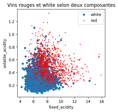
On ne garde que les deux premières.

X_train2 = X_train.iloc[:, :2]

import pandas

df = pandas.DataFrame(X_train2.copy())
df["y"] = y_train

import matplotlib.pyplot as plt

fig, ax = plt.subplots(1, 1, figsize=(4, 4))
df[df.y == "white"].plot(
    x="fixed_acidity", y="volatile_acidity", ax=ax, kind="scatter", label="white"
)
df[df.y == "red"].plot(
    x="fixed_acidity",
    y="volatile_acidity",
    ax=ax,
    kind="scatter",
    label="red",
    color="red",
    s=2,
)
ax.set_title("Vins rouges et white selon deux composantes");

from sklearn.linear_model import LogisticRegression

model = LogisticRegression()
model.fit(X_train2, y_train == "white")

LogisticRegression()

In a Jupyter environment, please rerun this cell to show the HTML representation or trust the notebook.
On GitHub, the HTML representation is unable to render, please try loading this page with nbviewer.org.

model.coef_, model.intercept_

(array([[ -1.11120776, -11.79383309]]), array([13.83313405]))

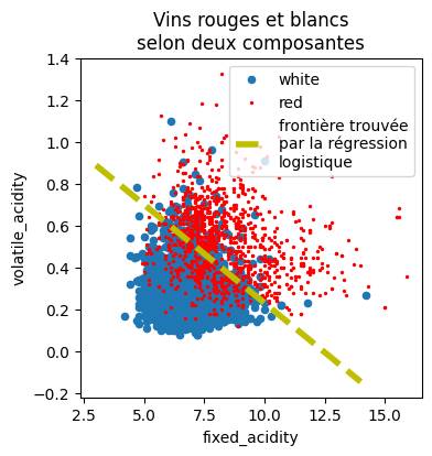
On trace cette droite sur le graphique.

x0 = 3
y0 = -(model.coef_[0, 0] * x0 + model.intercept_) / model.coef_[0, 1]
x1 = 14
y1 = -(model.coef_[0, 0] * x1 + model.intercept_) / model.coef_[0, 1]
x0, y0, x1, y1

(3, array([0.89025431]), 14, array([-0.14615898]))

import matplotlib.pyplot as plt

fig, ax = plt.subplots(1, 1, figsize=(4, 4))
df[df.y == "white"].plot(
    x="fixed_acidity", y="volatile_acidity", ax=ax, kind="scatter", label="white"
)
df[df.y == "red"].plot(
    x="fixed_acidity",
    y="volatile_acidity",
    ax=ax,
    kind="scatter",
    label="red",
    color="red",
    s=2,
)
ax.plot(
    [x0, x1],
    [y0, y1],
    "y--",
    lw=4,
    label="frontière trouvée\npar la régression\nlogistique",
)
ax.legend()
ax.set_title("Vins rouges et blancs\nselon deux composantes");

---

Notebook on github