Tree, hyperparamètres, overfitting#

L”overfitting ou surapprentissage apparaît lorsque les prédictions sur de nouvelles données sont nettement moins bonnes que celles obtenus sur la base d’apprentissage. Les forêts aléatoires sont moins sujettes à l’overfitting que les arbres de décisions qui les composent. Quelques illustrations.

[1]:

%matplotlib inline

Données générées#

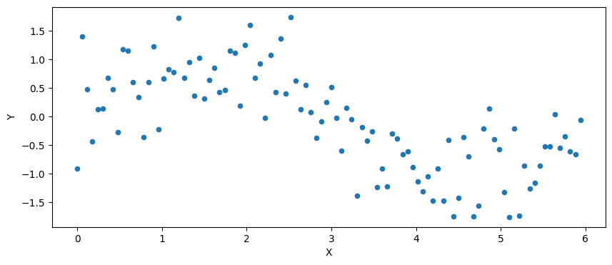
On génère un nuage de points $y_i = \sin(x_i) + \epsilon_i$ .

[2]:

import math
import pandas
import numpy, numpy.random


def generate_data(n):
    import matplotlib.pyplot as plt

    X = numpy.arange(n) / n * 6
    mat = numpy.random.normal(size=(n, 1)) / 2
    si = numpy.sin(X).reshape((n, 1))
    Y = mat + si
    X = X.reshape((n, 1))
    data = numpy.hstack((X, Y))
    return data, X, Y


n = 100
data, X, Y = generate_data(n)
df = pandas.DataFrame(data, columns=["X", "Y"])
df.plot(x="X", y="Y", kind="scatter", figsize=(10, 4));

../../_images/practice_ml_ml_a_tree_overfitting_3_0.png

Différents arbres de décision#

On regarde l’influence de paramêtres sur la sortie du modèle résultant de son apprentissage.

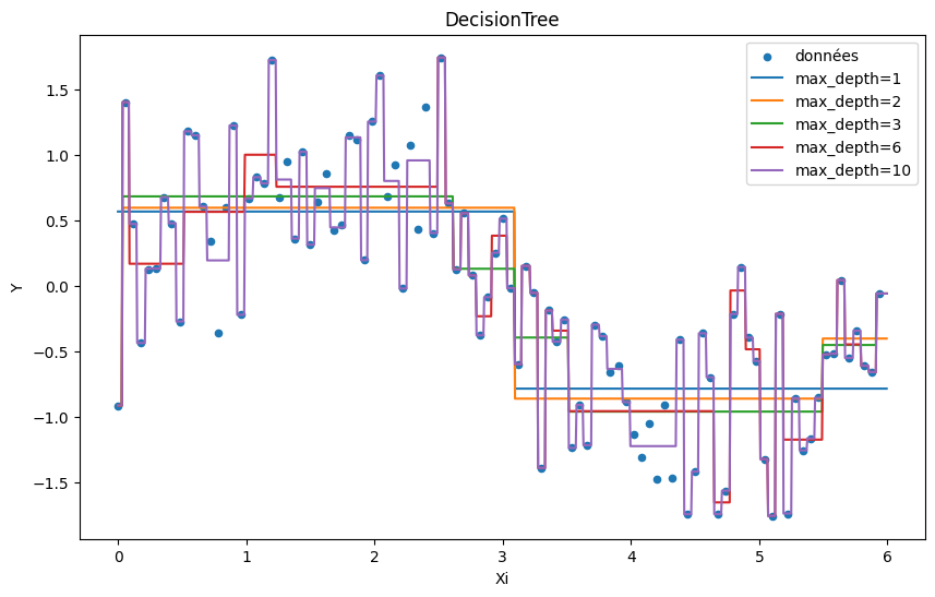
max_depth#

Un arbre représente une fonction en escalier. La profondeur détermine le nombre de feuilles, c’est-à-dire le nombre de valeurs possibles : $2^{max\_depth}$ .

[3]:

from sklearn.tree import DecisionTreeRegressor

ax = df.plot(
    x="X", y="Y", kind="scatter", figsize=(10, 6), label="données", title="DecisionTree"
)
Xi = (numpy.arange(n * 10) / n * 6 / 10).reshape((n * 10, 1))
for max_depth in [1, 2, 3, 6, 10]:
    clr = DecisionTreeRegressor(max_depth=max_depth)
    clr.fit(X, Y)
    pred = clr.predict(Xi)
    ex = pandas.DataFrame(Xi, columns=["Xi"])
    ex["pred"] = pred
    ex.sort_values("Xi").plot(
        x="Xi", y="pred", kind="line", label="max_depth=%d" % max_depth, ax=ax
    )

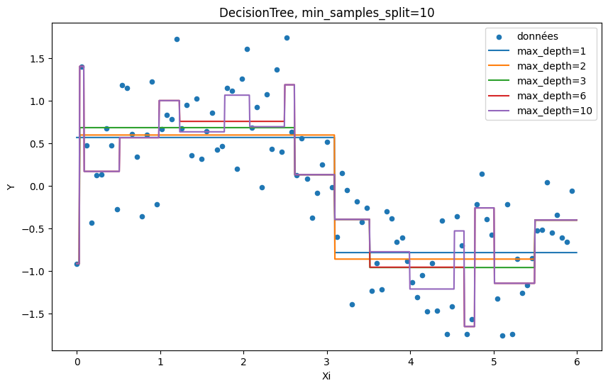
../../_images/practice_ml_ml_a_tree_overfitting_6_0.png

min_samples_split=10#

Chaque feuille d’un arbre prédit une valeur calculée à partir d’un ensemble d’observations. Ce nombre ne peut pas être inférieur à la valeur de ce paramètre. Ce mécanisme limite la possibilité de faire du surapprentissage en augmentant la représentativité de chaque feuille.

[4]:

ax = df.plot(
    x="X",
    y="Y",
    kind="scatter",
    figsize=(10, 6),
    label="données",
    title="DecisionTree, min_samples_split=10",
)
Xi = (numpy.arange(n * 10) / n * 6 / 10).reshape((n * 10, 1))
for max_depth in [1, 2, 3, 6, 10]:
    clr = DecisionTreeRegressor(max_depth=max_depth, min_samples_split=10)
    clr.fit(X, Y)
    pred = clr.predict(Xi)
    ex = pandas.DataFrame(Xi, columns=["Xi"])
    ex["pred"] = pred
    ex.sort_values("Xi").plot(
        x="Xi", y="pred", kind="line", label="max_depth=%d" % max_depth, ax=ax
    )

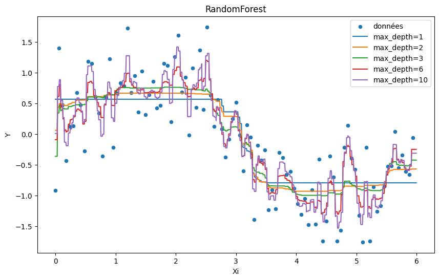
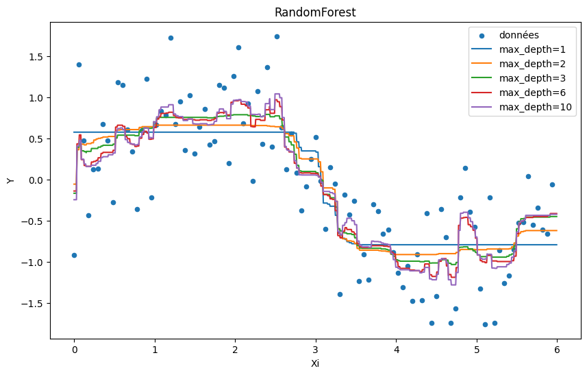
../../_images/practice_ml_ml_a_tree_overfitting_8_0.png

Random Forest#

On étudie les deux mêmes paramètres pour une random forest à ceci près que ce modèle est une somme pondérée des résultats produits par un ensemble d’arbres de décision.

max_depth#

[5]:

from sklearn.ensemble import RandomForestRegressor

ax = df.plot(
    x="X", y="Y", kind="scatter", figsize=(10, 6), label="données", title="RandomForest"
)
Xi = (numpy.arange(n * 10) / n * 6 / 10).reshape((n * 10, 1))
for max_depth in [1, 2, 3, 6, 10]:
    clr = RandomForestRegressor(max_depth=max_depth)
    clr.fit(X, Y.ravel())
    pred = clr.predict(Xi)
    ex = pandas.DataFrame(Xi, columns=["Xi"])
    ex["pred"] = pred
    ex.sort_values("Xi").plot(
        x="Xi", y="pred", kind="line", label="max_depth=%d" % max_depth, ax=ax
    )

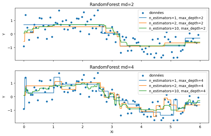
../../_images/practice_ml_ml_a_tree_overfitting_11_0.png

n_estimators#

n_estimators est le nombre d’itérations, c’est extactement le nombre d’arbres de décisions qui feront partie de la forêt dans le cas d’une régression ou d’une classification binaire.

[6]:

from sklearn.ensemble import RandomForestRegressor
import matplotlib.pyplot as plt

f, axarr = plt.subplots(2, sharex=True)
df.plot(
    x="X",
    y="Y",
    kind="scatter",
    figsize=(10, 6),
    label="données",
    title="RandomForest md=2",
    ax=axarr[0],
)
df.plot(
    x="X",
    y="Y",
    kind="scatter",
    figsize=(10, 6),
    label="données",
    title="RandomForest md=4",
    ax=axarr[1],
)
Xi = (numpy.arange(n * 10) / n * 6 / 10).reshape((n * 10, 1))
for i, max_depth in enumerate([2, 4]):
    for n_estimators in [1, 2, 10]:
        clr = RandomForestRegressor(n_estimators=n_estimators, max_depth=max_depth)
        clr.fit(X, Y.ravel())
        pred = clr.predict(Xi)
        ex = pandas.DataFrame(Xi, columns=["Xi"])
        ex["pred"] = pred
        ex.sort_values("Xi").plot(
            x="Xi",
            y="pred",
            kind="line",
            label="n_estimators=%d, max_depth=%d" % (n_estimators, max_depth),
            ax=axarr[i],
        )

../../_images/practice_ml_ml_a_tree_overfitting_13_0.png

min_samples_split=10#

[7]:

ax = df.plot(
    x="X", y="Y", kind="scatter", figsize=(10, 6), label="données", title="RandomForest"
)
Xi = (numpy.arange(n * 10) / n * 6 / 10).reshape((n * 10, 1))
for max_depth in [1, 2, 3, 6, 10]:
    clr = RandomForestRegressor(max_depth=max_depth, min_samples_split=10)
    clr.fit(X, Y.ravel())
    pred = clr.predict(Xi)
    ex = pandas.DataFrame(Xi, columns=["Xi"])
    ex["pred"] = pred
    ex.sort_values("Xi").plot(
        x="Xi", y="pred", kind="line", label="max_depth=%d" % max_depth, ax=ax
    )

../../_images/practice_ml_ml_a_tree_overfitting_15_0.png

Base d’apprentissage et et base de test#

C’est un des principes de base en machine learning : ne jamais tester un modèle sur les données d’apprentissage. Avec suffisamment de feuilles, un arbre de décision apprendra la valeur à prédire pour chaque observation. Le modèle apprend le bruit. Où s’arrête l’information, où commence le bruit, il n’est pas toujours évident de fixer le curseur.

Decision Tree#

[8]:

data, X, Y = generate_data(1000)

[9]:

from sklearn.model_selection import train_test_split

X_train, X_test, y_train, y_test = train_test_split(
    X, Y, test_size=0.33, random_state=42
)

[10]:

from sklearn.tree import DecisionTreeRegressor
from sklearn.metrics import r2_score

min_samples_splits = [2, 5, 10]
rows = []
for max_depth in range(1, 15):
    d = dict(max_depth=max_depth)
    for min_samples_split in min_samples_splits:
        clr = DecisionTreeRegressor(
            max_depth=max_depth, min_samples_split=min_samples_split
        )
        clr.fit(X_train, y_train)
        pred = clr.predict(X_test)
        score = r2_score(y_test, pred)
        d["min_samples_split=%d" % min_samples_split] = score
    rows.append(d)
pandas.DataFrame(rows).plot(
    x="max_depth", y=["min_samples_split=%d" % _ for _ in min_samples_splits]
);

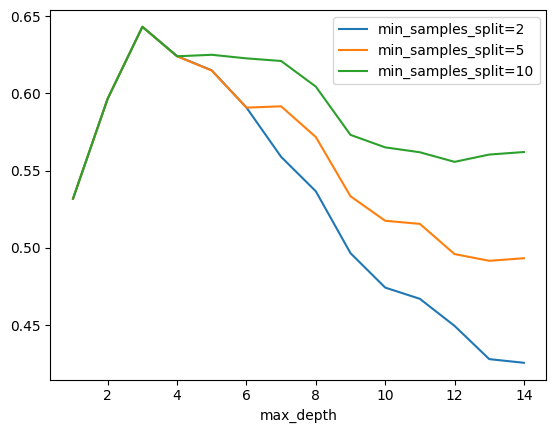
../../_images/practice_ml_ml_a_tree_overfitting_20_0.png

Le pic sur la base de test montre que passé un certain point, la performance décroît. A ce moment précis, le modèle commence à apprendre le bruit de la base d’apprentissage. Il overfitte. On remarque aussi que le modele overfitte moins lorsque min_samples_split=10.

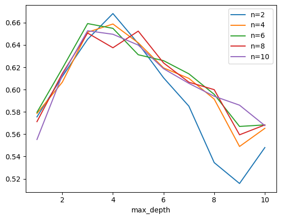
Random Forest#

[11]:

from sklearn.tree import DecisionTreeRegressor
from sklearn.metrics import r2_score

rows = []
for n_estimators in range(1, 11):
    for max_depth in range(1, 11):
        for min_samples_split in [2, 5, 10]:
            clr = RandomForestRegressor(n_estimators=n_estimators, max_depth=max_depth)
            clr.fit(X_train, y_train.ravel())
            pred = clr.predict(X_test)
            score = r2_score(y_test, pred)
            d = dict(max_depth=max_depth)
            d["n_estimators"] = n_estimators
            d["min_samples_split"] = min_samples_split
            d["score"] = score
            rows.append(d)
pl = pandas.DataFrame(rows)
pl.head()

[11]:

	max_depth	n_estimators	min_samples_split	score
0	1	1	2	0.521566
1	1	1	5	0.525835
2	1	1	10	0.534421
3	2	1	2	0.602039
4	2	1	5	0.585866

[12]:

ax = pl[(pl.min_samples_split == 10) & (pl.n_estimators == 2)].plot(
    x="max_depth", y="score", label="n=2"
)
for i in (4, 6, 8, 10):
    pl[(pl.min_samples_split == 10) & (pl.n_estimators == i)].plot(
        x="max_depth", y="score", label="n=%d" % i, ax=ax
    )

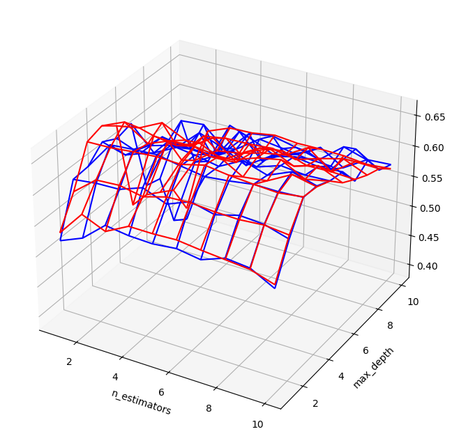
../../_images/practice_ml_ml_a_tree_overfitting_24_0.png

[13]:

import matplotlib.pyplot as plt
from mpl_toolkits.mplot3d import Axes3D

fig = plt.figure(figsize=(8, 8))
ax = fig.add_subplot(111, projection="3d")
for v, c in [(2, "b"), (10, "r")]:
    piv = pl[pl.min_samples_split == v].pivot(
        index="n_estimators", columns="max_depth", values="score"
    )
    pivX = piv.copy()
    pivY = piv.copy()
    for v in piv.columns:
        pivX.loc[:, v] = piv.index
    for v in piv.index:
        pivY.loc[v, :] = piv.columns
    ax.plot_wireframe(pivX.values, pivY.values, piv.values, color=c)
ax.set_xlabel("n_estimators")
ax.set_ylabel("max_depth");

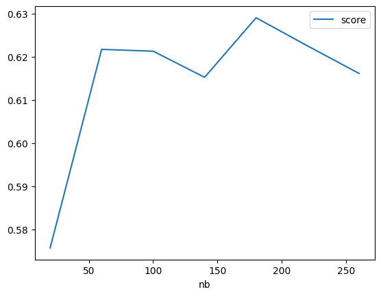
../../_images/practice_ml_ml_a_tree_overfitting_25_0.png

Réseaux de neurones#

Sur ce problème précis, les méthodes à base de gradient sont moins performantes. Elles paraissent également moins stables : la fonction d’erreur est plus agitée que celle obtenue pour les random forest. Ce type d’optimisation est plus sensible aux extrema locaux.

[14]:

from sklearn.neural_network import MLPRegressor
from sklearn.metrics import r2_score
from tqdm import tqdm

min_samples_splits = [2, 5, 10]
rows = []
for nb in tqdm(range(20, 300, 40)):
    clr = MLPRegressor(hidden_layer_sizes=(nb,), activation="relu", max_iter=200)
    clr.fit(X_train, y_train.ravel())
    pred = clr.predict(X_test)
    score = r2_score(y_test, pred)
    if score > 0:
        d = dict(nb=nb, score=score)
        rows.append(d)
pandas.DataFrame(rows).plot(x="nb", y=["score"]);

  0%|          | 0/7 [00:00<?, ?it/s] 29%|██▊       | 2/7 [00:03<00:09,  1.83s/it]/home/xadupre/install/scikit-learn/sklearn/neural_network/_multilayer_perceptron.py:691: ConvergenceWarning: Stochastic Optimizer: Maximum iterations (200) reached and the optimization hasn't converged yet.
  warnings.warn(
 43%|████▎     | 3/7 [00:07<00:10,  2.73s/it]/home/xadupre/install/scikit-learn/sklearn/neural_network/_multilayer_perceptron.py:691: ConvergenceWarning: Stochastic Optimizer: Maximum iterations (200) reached and the optimization hasn't converged yet.
  warnings.warn(
 57%|█████▋    | 4/7 [00:17<00:17,  5.89s/it]/home/xadupre/install/scikit-learn/sklearn/neural_network/_multilayer_perceptron.py:691: ConvergenceWarning: Stochastic Optimizer: Maximum iterations (200) reached and the optimization hasn't converged yet.
  warnings.warn(
 71%|███████▏  | 5/7 [00:24<00:12,  6.18s/it]/home/xadupre/install/scikit-learn/sklearn/neural_network/_multilayer_perceptron.py:691: ConvergenceWarning: Stochastic Optimizer: Maximum iterations (200) reached and the optimization hasn't converged yet.
  warnings.warn(
 86%|████████▌ | 6/7 [00:28<00:05,  5.32s/it]/home/xadupre/install/scikit-learn/sklearn/neural_network/_multilayer_perceptron.py:691: ConvergenceWarning: Stochastic Optimizer: Maximum iterations (200) reached and the optimization hasn't converged yet.
  warnings.warn(
100%|██████████| 7/7 [00:35<00:00,  5.03s/it]

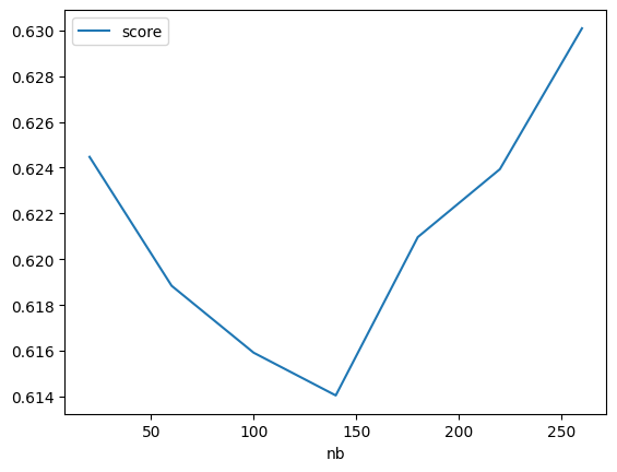
../../_images/practice_ml_ml_a_tree_overfitting_27_1.png

Réseaux de neurones, alpha=0#

[15]:

from sklearn.neural_network import MLPRegressor
from sklearn.metrics import r2_score

min_samples_splits = [2, 5, 10]
rows = []
for nb in tqdm(range(20, 300, 40)):
    clr = MLPRegressor(
        hidden_layer_sizes=(nb,), activation="relu", alpha=0, tol=1e-6, max_iter=200
    )
    clr.fit(X_train, y_train.ravel())
    pred = clr.predict(X_test)
    score = r2_score(y_test, pred)
    if score > 0:
        d = dict(nb=nb, score=score)
        rows.append(d)
pandas.DataFrame(rows).plot(x="nb", y=["score"]);

  0%|          | 0/7 [00:00<?, ?it/s]/home/xadupre/install/scikit-learn/sklearn/neural_network/_multilayer_perceptron.py:691: ConvergenceWarning: Stochastic Optimizer: Maximum iterations (200) reached and the optimization hasn't converged yet.
  warnings.warn(
 14%|█▍        | 1/7 [00:00<00:02,  2.18it/s]/home/xadupre/install/scikit-learn/sklearn/neural_network/_multilayer_perceptron.py:691: ConvergenceWarning: Stochastic Optimizer: Maximum iterations (200) reached and the optimization hasn't converged yet.
  warnings.warn(
 29%|██▊       | 2/7 [00:02<00:06,  1.34s/it]/home/xadupre/install/scikit-learn/sklearn/neural_network/_multilayer_perceptron.py:691: ConvergenceWarning: Stochastic Optimizer: Maximum iterations (200) reached and the optimization hasn't converged yet.
  warnings.warn(
 43%|████▎     | 3/7 [00:06<00:11,  2.80s/it]/home/xadupre/install/scikit-learn/sklearn/neural_network/_multilayer_perceptron.py:691: ConvergenceWarning: Stochastic Optimizer: Maximum iterations (200) reached and the optimization hasn't converged yet.
  warnings.warn(
 57%|█████▋    | 4/7 [00:13<00:13,  4.41s/it]/home/xadupre/install/scikit-learn/sklearn/neural_network/_multilayer_perceptron.py:691: ConvergenceWarning: Stochastic Optimizer: Maximum iterations (200) reached and the optimization hasn't converged yet.
  warnings.warn(
 71%|███████▏  | 5/7 [00:17<00:08,  4.24s/it]/home/xadupre/install/scikit-learn/sklearn/neural_network/_multilayer_perceptron.py:691: ConvergenceWarning: Stochastic Optimizer: Maximum iterations (200) reached and the optimization hasn't converged yet.
  warnings.warn(
 86%|████████▌ | 6/7 [00:21<00:03,  3.95s/it]/home/xadupre/install/scikit-learn/sklearn/neural_network/_multilayer_perceptron.py:691: ConvergenceWarning: Stochastic Optimizer: Maximum iterations (200) reached and the optimization hasn't converged yet.
  warnings.warn(
100%|██████████| 7/7 [00:24<00:00,  3.51s/it]

../../_images/practice_ml_ml_a_tree_overfitting_29_1.png

Exercice 1 : déterminer les paramètres optimaux pour cet exemple#

A vérifier avec grid_search, hyperopt, model_selection.

[ ]:

Exercice 2 : ajouter quelques points aberrants#

[ ]:

Intervalles de confiance#

On pourrait utiliser le module forest-confidence-interval mais il ne semble plus vraiment maintenu. Le module s’appuie sur le Jackknife pour estimer des intervalles de confiance. Il calcule un estimateur qui calcule une sortie en supprimant plusieurs fois un arbre lors de l’évaluation de la sortie de la forêt aléatoire. La théorie s’appuie sur un resampling de la base d’apprentissage que l’article considère comme équivalent à ceux effectués par scikit-learn pour générer chaque arbre. L’idée s’appuie sur l’article Confidence Intervals for Random Forests: The Jackknife and the Infinitesimal Jackknife.

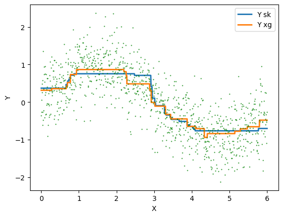
XGBoost#

[16]:

clr = RandomForestRegressor(n_estimators=10, max_depth=2)
clr.fit(X_train, y_train.ravel())

[16]:

RandomForestRegressor(max_depth=2, n_estimators=10)

In a Jupyter environment, please rerun this cell to show the HTML representation or trust the notebook.
On GitHub, the HTML representation is unable to render, please try loading this page with nbviewer.org.

[17]:

from xgboost import XGBRegressor

clrx = XGBRegressor(n_estimators=10, max_depth=2)
clrx.fit(X_train, y_train.ravel())

[17]:

XGBRegressor(base_score=None, booster=None, callbacks=None,
             colsample_bylevel=None, colsample_bynode=None,
             colsample_bytree=None, device=None, early_stopping_rounds=None,
             enable_categorical=False, eval_metric=None, feature_types=None,
             gamma=None, grow_policy=None, importance_type=None,
             interaction_constraints=None, learning_rate=None, max_bin=None,
             max_cat_threshold=None, max_cat_to_onehot=None,
             max_delta_step=None, max_depth=2, max_leaves=None,
             min_child_weight=None, missing=nan, monotone_constraints=None,
             multi_strategy=None, n_estimators=10, n_jobs=None,
             num_parallel_tree=None, random_state=None, ...)

[18]:

Xs = numpy.arange(start=0, stop=6, step=0.001)
Xs = Xs.reshape((len(Xs), 1))
ps = clr.predict(Xs)
ps = ps.reshape((len(ps), 1))
psx = clrx.predict(Xs)
psx = psx.reshape((len(psx), 1))

df = pandas.DataFrame(numpy.hstack((Xs, ps, psx)), columns=["X", "Y sk", "Y xg"])
ax = df.plot(x="X", y=["Y sk", "Y xg"], kind="line", lw=2)
ax.plot(X, Y, "g.", ms=1)
plt.xlabel("X")
plt.ylabel("Y");

../../_images/practice_ml_ml_a_tree_overfitting_38_0.png

Exercice 3 : optimiser les hyperparamètres pour XGBoost et scikit-learn et comparer#

[ ]:

Notebook on github