Valeurs manquantes et factorisation de matrices
Réflexion autour des valeur manquantes et de la factorisation de matrice positive.
[2]:
%matplotlib inline
Matrice à coefficients aléatoires
On étudie la factorisation d’une matrice à coefficients tout à fait aléatoires qui suivent une loi uniforme sur l’intervalle ![[0,1]](../../_images/math/5d6ef4de3a9f851a29bfae0016b7eadafffd99d7.svg) . Essayons sur une petite matrice :
. Essayons sur une petite matrice :
[3]:
from numpy.random import rand

M = rand(3, 3)
M
[3]:
array([[ 0.05119593,  0.43722929,  0.9290821 ],
       [ 0.4588466 ,  0.14187813,  0.23762633],
       [ 0.9768084 ,  0.47674026,  0.79044526]])
[4]:
from sklearn.decomposition import NMF

mf = NMF(1)
mf.fit_transform(M)
[4]:
array([[ 0.67825803],
       [ 0.38030919],
       [ 1.02295362]])
La matrice précédente est la matrice  dans le produit
  , la matrice qui suit est
  .
.
[5]:
mf.components_
[5]:
array([[ 0.73190904, 0.50765757, 0.92611883]])
[6]:
mf.reconstruction_err_ / (M.shape[0] * M.shape[1])
[6]:
0.07236890712696428
On recalcule l’erreur :
[7]:
d = M - mf.fit_transform(M) @ mf.components_
a = d.ravel()
e = a @ a.T
e**0.5 / (M.shape[0] * M.shape[1])
[7]:
0.072368907126964283
[8]:
e.ravel()
[8]:
array([ 0.42421796])
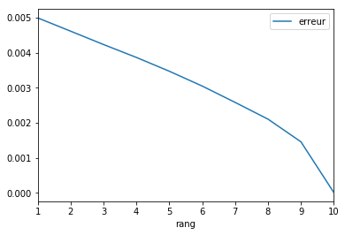
Et maintenant sur une grande et plus nécessairement carrée :
[9]:
M = rand(300, 10)
mf = NMF(1)
mf.fit_transform(M)
mf.reconstruction_err_ / (M.shape[0] * M.shape[1])
[9]:
0.004996164872801101
L’erreur est la même :
[10]:
errs = []
rangs = list(range(1, 11))
for k in rangs:
    mf = NMF(k)
    mf.fit_transform(M)
    e = mf.reconstruction_err_ / (M.shape[0] * M.shape[1])
    errs.append(e)
[11]:
import pandas

df = pandas.DataFrame(dict(rang=rangs, erreur=errs))
df.plot(x="rang", y="erreur")
[11]:
<matplotlib.axes._subplots.AxesSubplot at 0x199924d8668>
Matrice avec des vecteurs colonnes corrélés
Supposons maintenant que la matrice précédente  est de rang 3. Pour s’en assurer, on tire une matrice aléalatoire avec 3 vecteurs colonnes et on réplique des colonnes jusqu’à la dimension souhaitée.
[12]:
from numpy import hstack

M = rand(300, 3)
M = hstack([M, M, M, M[:, :1]])
M.shape
[12]:
(300, 10)
[13]:
errs = []
rangs = list(range(1, 11))
for k in rangs:
    mf = NMF(k)
    mf.fit_transform(M)
    e = mf.reconstruction_err_ / (M.shape[0] * M.shape[1])
    errs.append(e)
[14]:
import pandas

df = pandas.DataFrame(dict(rang=rangs, erreur=errs))
df.plot(x="rang", y="erreur")
[14]:
<matplotlib.axes._subplots.AxesSubplot at 0x199925d6630>
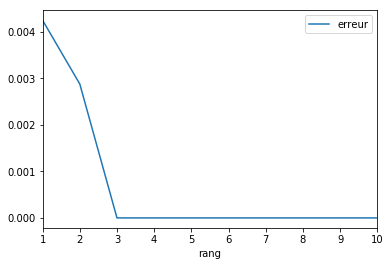
On essaye à nouveausur une matrice un peu plus petite.
[15]:
M = rand(3, 2)
M = hstack([M, M[:, :1]])
M
[15]:
array([[ 0.27190312,  0.6497563 ,  0.27190312],
       [ 0.44853292,  0.87097224,  0.44853292],
       [ 0.29424835,  0.65106952,  0.29424835]])
[16]:
mf = NMF(2)
mf.fit_transform(M)
[16]:
array([[ 0.61835197,  0.        ],
       [ 0.82887888,  0.29866219],
       [ 0.61960446,  0.07743224]])
[17]:
mf.components_
[17]:
array([[ 0.43972536,  1.05078419,  0.43972536],
       [ 0.28143493,  0.        ,  0.28143493]])
La dernière colonne est identique à la première.
Matrice identité
Et maintenant si la matrice est la matrice identité, que se passe-t-il ?
[18]:
from numpy import identity

M = identity(3)
M
[18]:
array([[ 1.,  0.,  0.],
       [ 0.,  1.,  0.],
       [ 0.,  0.,  1.]])
[19]:
mf = NMF(1)
mf.fit_transform(M)
[19]:
array([[ 0.],
       [ 1.],
       [ 0.]])
[20]:
mf.components_
[20]:
array([[ 0., 1., 0.]])
[21]:
mf.reconstruction_err_**2
[21]:
2.0000000000000004
On essaye avec  .
.
[22]:
mf = NMF(2)
mf.fit_transform(M)
[22]:
array([[ 0.        ,  0.        ],
       [ 0.        ,  1.03940448],
       [ 0.95521772,  0.        ]])
[23]:
mf.components_
[23]:
array([[ 0.        ,  0.        ,  1.04688175],
       [ 0.        ,  0.96208937,  0.        ]])
[24]:
mf.reconstruction_err_**2
[24]:
1.0
Avec des vecteurs normés et indépendants (formant donc une base de l’espace vectoriel), l’algorithme aboutit à une matrice égale au  premiers vecteurs et oublie les autres.
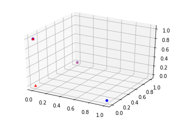
Matrice identité et représentation spatiale
Pour comprendre un peu mieux ce dernier exemple, il est utile de chercher d’autres solutions dont l’erreur est équivalente.
[25]:
def erreur_mf(M, W, H):
    d = M - W @ H
    a = d.ravel()
    e = a @ a.T
    e**0.5 / (M.shape[0] * M.shape[1])
    return e


M = identity(3)
mf = NMF(2)
W = mf.fit_transform(M)
H = mf.components_
erreur_mf(M, W, H)
[25]:
1.0
[26]:
W
[26]:
array([[ 0.        ,  0.        ],
       [ 0.9703523 ,  0.        ],
       [ 0.        ,  1.02721047]])
[27]:
H
[27]:
array([[ 0.        ,  1.03055354,  0.        ],
       [ 0.        ,  0.        ,  0.97351032]])
[28]:
W @ H
[28]:
array([[ 0.,  0.,  0.],
       [ 0.,  1.,  0.],
       [ 0.,  0.,  1.]])
[29]:
import matplotlib.pyplot as plt

fig = plt.figure()
ax = fig.add_subplot(111, projection="3d")
wh = W @ H
ax.scatter(M[:, 0], M[:, 1], M[:, 2], c="b", marker="o", s=20)
ax.scatter(wh[:, 0], wh[:, 1], wh[:, 2], c="r", marker="^")
[29]:
<mpl_toolkits.mplot3d.art3d.Path3DCollection at 0x19992d2a5c0>
Et si on pose maintenant :
[30]:
import numpy

W = numpy.array([[0.5, 0.5, 0], [0, 0, 1]]).T
H = numpy.array([[1, 1, 0], [0.0, 0.0, 1.0]])
W
[30]:
array([[ 0.5,  0. ],
       [ 0.5,  0. ],
       [ 0. ,  1. ]])
[31]:
H
[31]:
array([[ 1.,  1.,  0.],
       [ 0.,  0.,  1.]])
[32]:
W @ H
[32]:
array([[ 0.5,  0.5,  0. ],
       [ 0.5,  0.5,  0. ],
       [ 0. ,  0. ,  1. ]])
[33]:
erreur_mf(M, W, H)
[33]:
1.0
[34]:
fig = plt.figure()
ax = fig.add_subplot(111, projection="3d")
wh = W @ H
ax.scatter(M[:, 0], M[:, 1], M[:, 2], c="b", marker="o", s=20)
ax.scatter(wh[:, 0], wh[:, 1], wh[:, 2], c="r", marker="^")
[34]:
<mpl_toolkits.mplot3d.art3d.Path3DCollection at 0x19992a2e5f8>
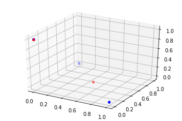
On peut voir la matrice comme un ensemble de  points dans un espace vectoriel. La matrice est un ensemble de
  points dans le même espace. La matrice , de rang est une approximation de cet ensemble dans le même espace, c’est aussi combinaisons linéaires de points de façon à former points les plus proches proches de points de la matrice .
[35]: