NeuralTreeNet et ONNX
La conversion d’un arbre de décision au format ONNX peut créer des différences entre le modèle original et le modèle converti (voir Issues when switching to float. Le problème vient d’un changement de type, les seuils de décisions sont arrondis au float32 le plus proche de leur valeur en float64 (double). Qu’advient-il si l’arbre de décision est converti en réseau de neurones d’abord.
L’approximation des seuils de décision ne change pas grand chose dans la majorité des cas. Cependant, il est possible que la comparaison d’une variable à un seuil de décision arrondi soit l’opposé de celle avec le seuil non arrondi. Dans ce cas, la décision suit un chemin différent dans l’arbre.
[1]:
%matplotlib inline
Jeu de données
On construit un jeu de donnée aléatoire.
[2]:
import numpy

X = numpy.random.randn(10000, 10)
y = X.sum(axis=1) / X.shape[1]
X = X.astype(numpy.float64)
y = y.astype(numpy.float64)
[3]:
middle = X.shape[0] // 2
X_train, X_test = X[:middle], X[middle:]
y_train, y_test = y[:middle], y[middle:]
Partie scikit-learn
Caler un arbre de décision
[4]:
from sklearn.tree import DecisionTreeRegressor

tree = DecisionTreeRegressor(max_depth=7)
tree.fit(X_train, y_train)
tree.score(X_train, y_train), tree.score(X_test, y_test)
[4]:
(0.6168207374163092, 0.35236821090506987)
[5]:
from sklearn.metrics import r2_score

r2_score(y_test, tree.predict(X_test))
[5]:
0.35236821090506987
La profondeur de l’arbre est insuffisante mais ce n’est pas ce qui nous intéresse ici.
Conversion au format ONNX
[6]:
from skl2onnx import to_onnx

onx = to_onnx(tree, X[:1].astype(numpy.float32))
[7]:
from onnxruntime import InferenceSession

x_exp = X_test

oinf = InferenceSession(onx.SerializeToString())
expected = tree.predict(x_exp)

got = oinf.run(None, {"X": x_exp.astype(numpy.float32)})[0]
numpy.abs(got - expected).max()
[7]:
np.float64(1.7091389654766018)
[8]:
from onnx_array_api.plotting.text_plot import onnx_simple_text_plot

print(onnx_simple_text_plot(onx))
opset: domain='ai.onnx.ml' version=1
opset: domain='' version=21
opset: domain='' version=21
input: name='X' type=dtype('float32') shape=['', 10]
TreeEnsembleRegressor(X, n_targets=1, nodes_falsenodeids=255:[128,65,34...254,0,0], nodes_featureids=255:[3,4,0...4,0,0], nodes_hitrates=255:[1.0,1.0...1.0,1.0], nodes_missing_value_tracks_true=255:[0,0,0...0,0,0], nodes_modes=255:[b'BRANCH_LEQ',b'BRANCH_LEQ'...b'LEAF',b'LEAF'], nodes_nodeids=255:[0,1,2...252,253,254], nodes_treeids=255:[0,0,0...0,0,0], nodes_truenodeids=255:[1,2,3...253,0,0], nodes_values=255:[0.12306099385023117,-0.19721701741218567...0.0,0.0], post_transform=b'NONE', target_ids=128:[0,0,0...0,0,0], target_nodeids=128:[7,8,10...251,253,254], target_treeids=128:[0,0,0...0,0,0], target_weights=128:[-0.9612963795661926,-0.5883080959320068...0.49337825179100037,0.7387731075286865]) -> variable
output: name='variable' type=dtype('float32') shape=['', 1]
Après la conversion en un réseau de neurones
Conversion en un réseau de neurones
Un paramètre permet de faire varier la pente des fonctions sigmoïdes utilisées.
[9]:
from tqdm import tqdm
from pandas import DataFrame
from mlstatpy.ml.neural_tree import NeuralTreeNet

xe = x_exp[:500]
expected = tree.predict(xe)

data = []
trees = {}
for i in tqdm([0.3, 0.4, 0.5, 0.7, 0.9, 1] + list(range(5, 61, 5))):
    root = NeuralTreeNet.create_from_tree(tree, k=i, arch="compact")
    got = root.predict(xe)[:, -1]
    me = numpy.abs(got - expected).mean()
    mx = numpy.abs(got - expected).max()
    obs = dict(k=i, max=mx, mean=me)
    data.append(obs)
    trees[i] = root
100%|██████████| 18/18 [00:00<00:00, 53.66it/s]
[10]:
df = DataFrame(data)
df
[10]:
| k | max | mean | |
|---|---|---|---|
| 0 | 0.3 | 0.890666 | 0.212437 |
| 1 | 0.4 | 0.586997 | 0.141997 |
| 2 | 0.5 | 0.520952 | 0.129502 |
| 3 | 0.7 | 0.588261 | 0.127598 |
| 4 | 0.9 | 0.579515 | 0.123064 |
| 5 | 1.0 | 0.599704 | 0.119385 |
| 6 | 5.0 | 0.486386 | 0.021135 |
| 7 | 10.0 | 0.485185 | 0.005929 |
| 8 | 15.0 | 0.325395 | 0.002471 |
| 9 | 20.0 | 0.309316 | 0.001763 |
| 10 | 25.0 | 0.214692 | 0.000968 |
| 11 | 30.0 | 0.214629 | 0.000846 |
| 12 | 35.0 | 0.163406 | 0.000659 |
| 13 | 40.0 | 0.069112 | 0.000268 |
| 14 | 45.0 | 0.064403 | 0.000214 |
| 15 | 50.0 | 0.059307 | 0.000172 |
| 16 | 55.0 | 0.053915 | 0.000140 |
| 17 | 60.0 | 0.048336 | 0.000114 |
[11]:
df.set_index("k").plot(title="Précision de la conversion\nen réseau de neurones");
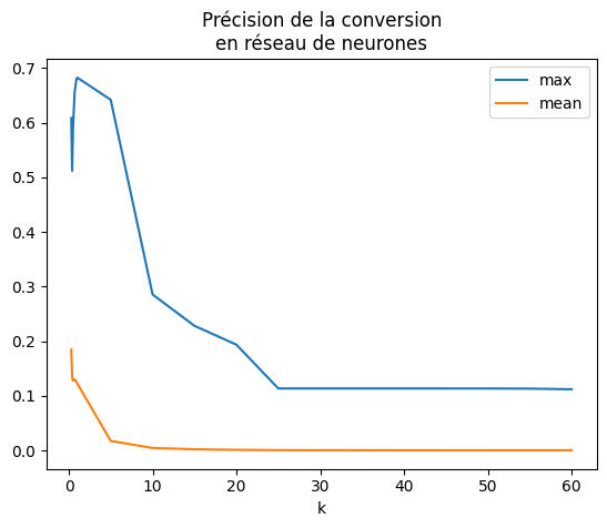
L’erreur est meilleure mais il faudrait recommencer l’expérience plusieurs fois avant de pouvoir conclure afin d’obtenir un interval de confiance pour le même type de jeu de données. Ce sera pour une autre fois. Le résultat dépend du jeu de données et surtout de la proximité des seuils de décisions. Néanmoins, on calcule l’erreur sur l’ensemble de la base de test. Celle-ci a été tronquée pour aller plus vite.
[12]:
expected = tree.predict(x_exp)
got = trees[50].predict(x_exp)[:, -1]
numpy.abs(got - expected).max(), numpy.abs(got - expected).mean()
[12]:
(np.float64(0.14867156347163313), np.float64(0.00014171388788628532))
On voit que l’erreur peut-être très grande. Elle reste néanmoins plus petite que l’erreur de conversion introduite par ONNX.
Conversion au format ONNX
On crée tout d’abord une classe qui suit l’API de scikit-learn et qui englobe l’arbre qui vient d’être créé qui sera ensuite convertit en ONNX.
[13]:
from mlstatpy.ml.neural_tree import NeuralTreeNetRegressor

reg = NeuralTreeNetRegressor(trees[50])
onx2 = to_onnx(reg, X[:1].astype(numpy.float32))
[14]:
print(onnx_simple_text_plot(onx2))
opset: domain='' version=21
input: name='X' type=dtype('float32') shape=['', 10]
init: name='Ma_MatMulcst' type=float32 shape=(10, 127)
init: name='Ad_Addcst' type=float32 shape=(127,)
init: name='Mu_Mulcst' type=float32 shape=(1,) -- array([4.], dtype=float32)
init: name='Ma_MatMulcst1' type=float32 shape=(127, 128)
init: name='Ad_Addcst1' type=float32 shape=(128,)
init: name='Ma_MatMulcst2' type=float32 shape=(128, 1)
init: name='Ad_Addcst2' type=float32 shape=(1,) -- array([0.], dtype=float32)
MatMul(X, Ma_MatMulcst) -> Ma_Y02
  Add(Ma_Y02, Ad_Addcst) -> Ad_C02
    Mul(Ad_C02, Mu_Mulcst) -> Mu_C01
      Sigmoid(Mu_C01) -> Si_Y01
        MatMul(Si_Y01, Ma_MatMulcst1) -> Ma_Y01
          Add(Ma_Y01, Ad_Addcst1) -> Ad_C01
            Mul(Ad_C01, Mu_Mulcst) -> Mu_C0
              Sigmoid(Mu_C0) -> Si_Y0
                MatMul(Si_Y0, Ma_MatMulcst2) -> Ma_Y0
                  Add(Ma_Y0, Ad_Addcst2) -> Ad_C0
                    Identity(Ad_C0) -> variable
output: name='variable' type=dtype('float32') shape=['', 1]
[15]:
oinf2 = InferenceSession(
    onx2.SerializePartialToString(), providers=["CPUExecutionProvider"]
)
expected = tree.predict(x_exp)

got = oinf2.run(["variable"], {"X": x_exp.astype(numpy.float32)})[0]
numpy.abs(got - expected).max()
[15]:
np.float64(1.7091389654766018)
L’erreur est la même.
Temps de calcul
[16]:
x_exp32 = x_exp.astype(numpy.float32)
Tout d’abord le temps de calcul pour scikit-learn.
[17]:
%timeit tree.predict(x_exp32)
312 μs ± 9.06 μs per loop (mean ± std. dev. of 7 runs, 1,000 loops each)
Le temps de calcul pour l’arbre de décision au format ONNX.
[18]:
%timeit oinf.run(None, {'X': x_exp32})[0]
35 μs ± 595 ns per loop (mean ± std. dev. of 7 runs, 10,000 loops each)
Et le temps de calcul pour le réseau de neurones au format ONNX.m
[19]:
%timeit oinf2.run(None, {'X': x_exp32})[0]
1.18 ms ± 7.98 μs per loop (mean ± std. dev. of 7 runs, 1,000 loops each)
Ce temps de calcul très long est attendu car le modèle contient une multiplication de matrice très grande et surtout que tous les seuils de l’arbre sont calculés pour chaque observation. Là où l’implémentation de l’arbre de décision calcule d seuils, la profondeur de l’arbre, la nouvelle implémentation calcule tous les seuils soit  pour chaque feuille. Il y a feuilles. Même en étant sparse, on peut réduire les calculs à
  ce qui fait encore beaucoup de
calculs inutiles.
ce qui fait encore beaucoup de
calculs inutiles.
[20]:
for node in trees[50].nodes:
    print(node.coef.shape, node.bias.shape)
(127, 11) (127,)
(128, 128) (128,)
(129,) ()
Cela dit, la plus grande matrice est creuse, elle peut être réduite considérablement.
[21]:
from scipy.sparse import csr_matrix

for node in trees[50].nodes:
    csr = csr_matrix(node.coef)
    print(
        f"coef.shape={node.coef.shape}, size dense={node.coef.size}, "
        f"size sparse={csr.size}, ratio={csr.size / node.coef.size}"
    )
coef.shape=(127, 11), size dense=1397, size sparse=254, ratio=0.18181818181818182
coef.shape=(128, 128), size dense=16384, size sparse=1024, ratio=0.0625
coef.shape=(129,), size dense=129, size sparse=128, ratio=0.9922480620155039
[22]:
r = numpy.random.randn(trees[50].nodes[1].coef.shape[0])
mat = trees[50].nodes[1].coef
%timeit mat @ r
2.87 μs ± 177 ns per loop (mean ± std. dev. of 7 runs, 100,000 loops each)
[23]:
csr = csr_matrix(mat)
%timeit csr @ r
3.53 μs ± 88.3 ns per loop (mean ± std. dev. of 7 runs, 100,000 loops each)
Ce serait beaucoup plus rapide avec une matrice sparse et d’autant plus rapide que l’arbre est profond. Le modèle ONNX se décompose comme suit.
[24]:
print(onnx_simple_text_plot(onx2))
opset: domain='' version=21
input: name='X' type=dtype('float32') shape=['', 10]
init: name='Ma_MatMulcst' type=float32 shape=(10, 127)
init: name='Ad_Addcst' type=float32 shape=(127,)
init: name='Mu_Mulcst' type=float32 shape=(1,) -- array([4.], dtype=float32)
init: name='Ma_MatMulcst1' type=float32 shape=(127, 128)
init: name='Ad_Addcst1' type=float32 shape=(128,)
init: name='Ma_MatMulcst2' type=float32 shape=(128, 1)
init: name='Ad_Addcst2' type=float32 shape=(1,) -- array([0.], dtype=float32)
MatMul(X, Ma_MatMulcst) -> Ma_Y02
  Add(Ma_Y02, Ad_Addcst) -> Ad_C02
    Mul(Ad_C02, Mu_Mulcst) -> Mu_C01
      Sigmoid(Mu_C01) -> Si_Y01
        MatMul(Si_Y01, Ma_MatMulcst1) -> Ma_Y01
          Add(Ma_Y01, Ad_Addcst1) -> Ad_C01
            Mul(Ad_C01, Mu_Mulcst) -> Mu_C0
              Sigmoid(Mu_C0) -> Si_Y0
                MatMul(Si_Y0, Ma_MatMulcst2) -> Ma_Y0
                  Add(Ma_Y0, Ad_Addcst2) -> Ad_C0
                    Identity(Ad_C0) -> variable
output: name='variable' type=dtype('float32') shape=['', 1]
Voyons comment le temps de calcul se répartit.
[25]:
from onnxruntime import InferenceSession, SessionOptions
from onnx_diagnostic.helpers.rt_helper import js_profile_to_dataframe

sess_options = SessionOptions()
sess_options.enable_profiling = True

sess = InferenceSession(
    onx2.SerializeToString(), sess_options, providers=["CPUExecutionProvider"]
)
for i in range(43):
    sess.run(None, {"X": x_exp32})

prof = sess.end_profiling()
[26]:
df = js_profile_to_dataframe(prof, first_it_out=True)
df
[26]:
| cat | pid | tid | dur | ts | ph | name | args_thread_scheduling_stats | args_output_size | args_parameter_size | args_activation_size | args_node_index | args_provider | args_op_name | op_name | event_name | iteration | it==0 | |
|---|---|---|---|---|---|---|---|---|---|---|---|---|---|---|---|---|---|---|
| 0 | Session | 50840 | 50840 | 458 | 9 | X | model_loading_array | NaN | NaN | NaN | NaN | NaN | NaN | NaN | NaN | model_loading_array | -1 | 1 |
| 1 | Session | 50840 | 50840 | 1365 | 529 | X | session_initialization | NaN | NaN | NaN | NaN | NaN | NaN | NaN | NaN | session_initialization | -1 | 1 |
| 2 | Node | 50840 | 50840 | 3437 | 2343 | X | Ma_MatMul/MatMulAddFusion_kernel_time | {'main_thread': {'thread_pool_name': 'session-... | 2540000 | 508 | 200000 | 11 | CPUExecutionProvider | Gemm | Ma_MatMul/MatMulAddFusion | kernel_time | -1 | 1 |
| 3 | Node | 50840 | 50840 | 776 | 5808 | X | Mu_Mul_kernel_time | {'main_thread': {'thread_pool_name': 'session-... | 2540000 | 4 | 2540000 | 2 | CPUExecutionProvider | Mul | Mu_Mul | kernel_time | -1 | 1 |
| 4 | Node | 50840 | 50840 | 130 | 6604 | X | Si_Sigmoid_kernel_time | {'main_thread': {'thread_pool_name': 'session-... | 2540000 | 0 | 2540000 | 3 | CPUExecutionProvider | Sigmoid | Si_Sigmoid | kernel_time | -1 | 1 |
| ... | ... | ... | ... | ... | ... | ... | ... | ... | ... | ... | ... | ... | ... | ... | ... | ... | ... | ... |
| 384 | Node | 50840 | 50840 | 52 | 134871 | X | Mu_Mul1_kernel_time | {'main_thread': {'thread_pool_name': 'session-... | 2560000 | 4 | 2560000 | 6 | CPUExecutionProvider | Mul | Mu_Mul1 | kernel_time | 41 | 0 |
| 385 | Node | 50840 | 50840 | 72 | 134943 | X | Si_Sigmoid1_kernel_time | {'main_thread': {'thread_pool_name': 'session-... | 2560000 | 0 | 2560000 | 7 | CPUExecutionProvider | Sigmoid | Si_Sigmoid1 | kernel_time | 41 | 0 |
| 386 | Node | 50840 | 50840 | 79 | 135022 | X | Ma_MatMul2_kernel_time | {'main_thread': {'thread_pool_name': 'session-... | 20000 | 0 | 2560000 | 8 | CPUExecutionProvider | MatMul | Ma_MatMul2 | kernel_time | 41 | 0 |
| 387 | Session | 50840 | 50840 | 1508 | 133600 | X | SequentialExecutor::Execute | NaN | NaN | NaN | NaN | NaN | NaN | NaN | NaN | SequentialExecutor::Execute | 42 | 0 |
| 388 | Session | 50840 | 50840 | 1523 | 133591 | X | model_run | NaN | NaN | NaN | NaN | NaN | NaN | NaN | NaN | model_run | 42 | 0 |
389 rows × 18 columns
[27]:
set(df["args_provider"])
[27]:
{'CPUExecutionProvider', nan}
[28]:
dfp = df[df.args_provider == "CPUExecutionProvider"].copy()
dfp["name"] = dfp["name"].apply(lambda s: s.replace("_kernel_time", ""))
gr_dur = (
    dfp[["dur", "args_op_name", "name"]]
    .groupby(["args_op_name", "name"])
    .sum()
    .sort_values("dur")
)
gr_dur
[28]:
| dur | ||
|---|---|---|
| args_op_name | name | |
| Mul | Mu_Mul1 | 6486 |
| Sigmoid | Si_Sigmoid1 | 7064 |
| Mul | Mu_Mul | 7401 |
| Sigmoid | Si_Sigmoid | 7594 |
| MatMul | Ma_MatMul2 | 8032 |
| Gemm | Ma_MatMul/MatMulAddFusion | 28069 |
| Ma_MatMul1/MatMulAddFusion | 55140 |
[29]:
gr_n = (
    dfp[["dur", "args_op_name", "name"]]
    .groupby(["args_op_name", "name"])
    .count()
    .sort_values("dur")
)
gr_n = gr_n.loc[gr_dur.index, :]
gr_n
[29]:
| dur | ||
|---|---|---|
| args_op_name | name | |
| Mul | Mu_Mul1 | 43 |
| Sigmoid | Si_Sigmoid1 | 43 |
| Mul | Mu_Mul | 43 |
| Sigmoid | Si_Sigmoid | 43 |
| MatMul | Ma_MatMul2 | 43 |
| Gemm | Ma_MatMul/MatMulAddFusion | 43 |
| Ma_MatMul1/MatMulAddFusion | 43 |
[30]:
import matplotlib.pyplot as plt

fig, ax = plt.subplots(1, 2, figsize=(12, 4))
gr_dur.plot.barh(ax=ax[0])
gr_n.plot.barh(ax=ax[1])
ax[0].set_title("duration")
ax[1].set_title("n occurences");
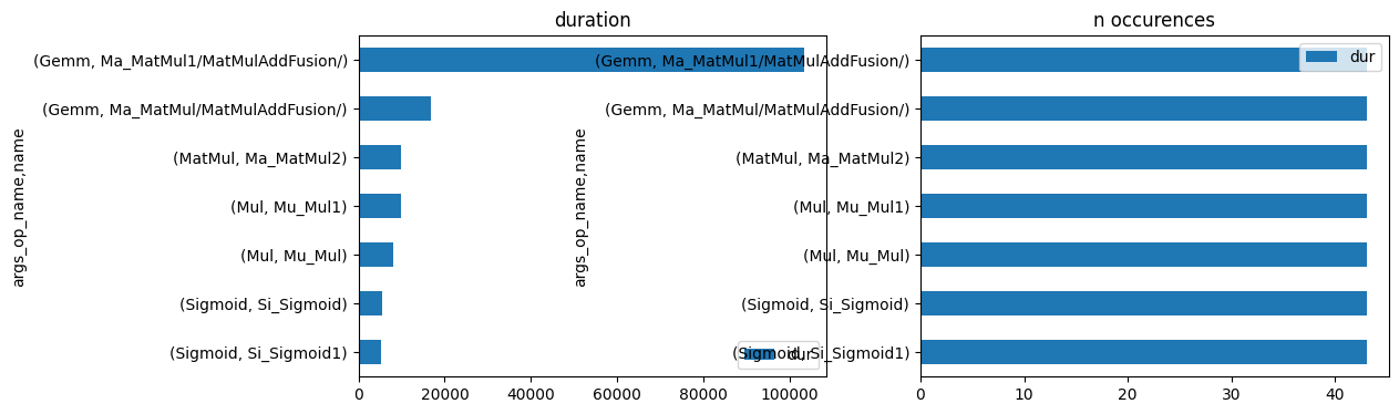
onnxruntime passe principalement son temps dans un produit matriciel. On vérifie plus précisément.
[31]:
df[(df.args_op_name == "Gemm") & (df.dur > 0)].sort_values("dur", ascending=False).head(
    n=2
).T
[31]:
| 11 | 2 | |
|---|---|---|
| cat | Node | Node |
| pid | 50840 | 50840 |
| tid | 50840 | 50840 |
| dur | 3549 | 3437 |
| ts | 10439 | 2343 |
| ph | X | X |
| name | Ma_MatMul/MatMulAddFusion_kernel_time | Ma_MatMul/MatMulAddFusion_kernel_time |
| args_thread_scheduling_stats | {'main_thread': {'thread_pool_name': 'session-... | {'main_thread': {'thread_pool_name': 'session-... |
| args_output_size | 2540000 | 2540000 |
| args_parameter_size | 508 | 508 |
| args_activation_size | 200000 | 200000 |
| args_node_index | 11 | 11 |
| args_provider | CPUExecutionProvider | CPUExecutionProvider |
| args_op_name | Gemm | Gemm |
| op_name | Ma_MatMul/MatMulAddFusion | Ma_MatMul/MatMulAddFusion |
| event_name | kernel_time | kernel_time |
| iteration | 0 | -1 |
| it==0 | 1 | 1 |
C’est un produit matriciel d’environ 5000x800 par 800x800.
[32]:
gr_dur / gr_dur.dur.sum()
[32]:
| dur | ||
|---|---|---|
| args_op_name | name | |
| Mul | Mu_Mul1 | 0.054147 |
| Sigmoid | Si_Sigmoid1 | 0.058972 |
| Mul | Mu_Mul | 0.061785 |
| Sigmoid | Si_Sigmoid | 0.063396 |
| MatMul | Ma_MatMul2 | 0.067053 |
| Gemm | Ma_MatMul/MatMulAddFusion | 0.234326 |
| Ma_MatMul1/MatMulAddFusion | 0.460321 |
[33]:
r = (gr_dur / gr_dur.dur.sum()).dur.max()
r
[33]:
np.float64(0.46032090561501343)
Il occupe 82% du temps. et d’après l’expérience précédente, son temps d’éxecution peut-être réduit par 10 en le remplaçant par une matrice sparse. Cela ne suffira pas pour accélerer le temps de calcul de ce réseau de neurones. Il est 84 ms comparé à 247 µs pour l’arbre de décision. Avec cette optimisation, il pourrait passer de :
[34]:
t = 3.75  # ms
t * (1 - r) + r * t / 12
[34]:
np.float64(2.167646886948391)
Soit une réduction du temps de calcul. Ce n’est pas mal mais pas assez.
Hummingbird
hummingbird est une librairie qui convertit un arbre de décision en réseau de neurones. Voyons ses performances.
[36]:
from hummingbird.ml import convert

model = convert(tree, "torch")

expected = tree.predict(x_exp)
got = model.predict(x_exp)
numpy.abs(got - expected).max(), numpy.abs(got - expected).mean()
[36]:
(np.float64(2.7422816128996885e-08), np.float64(3.844877509922521e-09))
Le résultat est beaucoup plus fidèle au modèle.
[37]:
%timeit model.predict(x_exp)
526 μs ± 41.2 μs per loop (mean ± std. dev. of 7 runs, 1,000 loops each)
Il reste plus lent mais beaucoup plus rapide que la solution manuelle proposée dans les précédents paragraphes. Il contient un attribut model.
[53]:
import torch

isinstance(model.model, torch.nn.Module)
[53]:
True
On convertit ce modèle au format ONNX.
[58]:
import torch.onnx

x = torch.randn(x_exp.shape[0], x_exp.shape[1], requires_grad=True)
torch.onnx.export(
    model.model,
    x,
    "tree_torch.onnx",
    opset_version=15,
    input_names=["X"],
    output_names=["variable"],
    dynamic_axes={"X": {0: "batch_size"}, "variable": {0: "batch_size"}},
    dynamo=False,
)
/tmp/ipykernel_50840/2369393440.py:4: DeprecationWarning: You are using the legacy TorchScript-based ONNX export. Starting in PyTorch 2.9, the new torch.export-based ONNX exporter has become the default. Learn more about the new export logic: https://docs.pytorch.org/docs/stable/onnx_export.html. For exporting control flow: https://pytorch.org/tutorials/beginner/onnx/export_control_flow_model_to_onnx_tutorial.html
  torch.onnx.export(
[59]:
import onnx

onxh = onnx.load("tree_torch.onnx")
[60]:
print(onnx_simple_text_plot(onxh, raise_exc=False))
opset: domain='' version=15
input: name='X' type=dtype('float32') shape=['batch_size', 10]
init: name='_operators.0.root_nodes' type=int64 shape=(1,) -- array([3])
init: name='_operators.0.root_biases' type=float32 shape=(1,) -- array([0.123061], dtype=float32)
init: name='_operators.0.tree_indices' type=int64 shape=(1,) -- array([0])
init: name='_operators.0.leaf_nodes' type=float32 shape=(128, 1)
init: name='_operators.0.nodes.0' type=int64 shape=(2,) -- array([2, 4])
init: name='_operators.0.nodes.1' type=int64 shape=(4,) -- array([5, 8, 1, 0])
init: name='_operators.0.nodes.2' type=int64 shape=(8,)
init: name='_operators.0.nodes.3' type=int64 shape=(16,)
init: name='_operators.0.nodes.4' type=int64 shape=(32,)
init: name='_operators.0.nodes.5' type=int64 shape=(64,)
init: name='_operators.0.biases.0' type=float32 shape=(2,) -- array([-0.00307798, -0.19721702], dtype=float32)
init: name='_operators.0.biases.1' type=float32 shape=(4,) -- array([ 0.04036466, -0.18311241,  0.2513926 , -0.7457566 ], dtype=float32)
init: name='_operators.0.biases.2' type=float32 shape=(8,)
init: name='_operators.0.biases.3' type=float32 shape=(16,)
init: name='_operators.0.biases.4' type=float32 shape=(32,)
init: name='_operators.0.biases.5' type=float32 shape=(64,)
Constant(value=[-1]) -> /_operators.0/Constant_output_0
Gather(X, _operators.0.root_nodes, axis=1) -> /_operators.0/Gather_output_0
  LessOrEqual(/_operators.0/Gather_output_0, _operators.0.root_biases) -> /_operators.0/LessOrEqual_output_0
    Cast(/_operators.0/LessOrEqual_output_0, to=7) -> /_operators.0/Cast_output_0
      Add(/_operators.0/Cast_output_0, _operators.0.tree_indices) -> /_operators.0/Add_output_0
  Reshape(/_operators.0/Add_output_0, /_operators.0/Constant_output_0, allowzero=0) -> /_operators.0/Reshape_output_0
    Gather(_operators.0.nodes.0, /_operators.0/Reshape_output_0, axis=0) -> /_operators.0/Gather_1_output_0
Constant(value=[-1, 1]) -> /_operators.0/Constant_1_output_0
  Reshape(/_operators.0/Gather_1_output_0, /_operators.0/Constant_1_output_0, allowzero=0) -> /_operators.0/Reshape_1_output_0
    GatherElements(X, /_operators.0/Reshape_1_output_0, axis=1) -> /_operators.0/GatherElements_output_0
Constant(value=[-1]) -> /_operators.0/Constant_2_output_0
  Reshape(/_operators.0/GatherElements_output_0, /_operators.0/Constant_2_output_0, allowzero=0) -> /_operators.0/Reshape_2_output_0
Constant(value=2) -> /_operators.0/Constant_3_output_0
  Mul(/_operators.0/Reshape_output_0, /_operators.0/Constant_3_output_0) -> /_operators.0/Mul_output_0
Gather(_operators.0.biases.0, /_operators.0/Reshape_output_0, axis=0) -> /_operators.0/Gather_2_output_0
  LessOrEqual(/_operators.0/Reshape_2_output_0, /_operators.0/Gather_2_output_0) -> /_operators.0/LessOrEqual_1_output_0
    Cast(/_operators.0/LessOrEqual_1_output_0, to=7) -> /_operators.0/Cast_1_output_0
    Add(/_operators.0/Mul_output_0, /_operators.0/Cast_1_output_0) -> /_operators.0/Add_1_output_0
      Gather(_operators.0.nodes.1, /_operators.0/Add_1_output_0, axis=0) -> /_operators.0/Gather_3_output_0
Constant(value=[-1, 1]) -> /_operators.0/Constant_4_output_0
  Reshape(/_operators.0/Gather_3_output_0, /_operators.0/Constant_4_output_0, allowzero=0) -> /_operators.0/Reshape_3_output_0
    GatherElements(X, /_operators.0/Reshape_3_output_0, axis=1) -> /_operators.0/GatherElements_1_output_0
Constant(value=[-1]) -> /_operators.0/Constant_5_output_0
  Reshape(/_operators.0/GatherElements_1_output_0, /_operators.0/Constant_5_output_0, allowzero=0) -> /_operators.0/Reshape_4_output_0
Constant(value=2) -> /_operators.0/Constant_6_output_0
  Mul(/_operators.0/Add_1_output_0, /_operators.0/Constant_6_output_0) -> /_operators.0/Mul_1_output_0
Gather(_operators.0.biases.1, /_operators.0/Add_1_output_0, axis=0) -> /_operators.0/Gather_4_output_0
  LessOrEqual(/_operators.0/Reshape_4_output_0, /_operators.0/Gather_4_output_0) -> /_operators.0/LessOrEqual_2_output_0
    Cast(/_operators.0/LessOrEqual_2_output_0, to=7) -> /_operators.0/Cast_2_output_0
    Add(/_operators.0/Mul_1_output_0, /_operators.0/Cast_2_output_0) -> /_operators.0/Add_2_output_0
      Gather(_operators.0.nodes.2, /_operators.0/Add_2_output_0, axis=0) -> /_operators.0/Gather_5_output_0
Constant(value=[-1, 1]) -> /_operators.0/Constant_7_output_0
  Reshape(/_operators.0/Gather_5_output_0, /_operators.0/Constant_7_output_0, allowzero=0) -> /_operators.0/Reshape_5_output_0
    GatherElements(X, /_operators.0/Reshape_5_output_0, axis=1) -> /_operators.0/GatherElements_2_output_0
Constant(value=[-1]) -> /_operators.0/Constant_8_output_0
  Reshape(/_operators.0/GatherElements_2_output_0, /_operators.0/Constant_8_output_0, allowzero=0) -> /_operators.0/Reshape_6_output_0
Constant(value=2) -> /_operators.0/Constant_9_output_0
  Mul(/_operators.0/Add_2_output_0, /_operators.0/Constant_9_output_0) -> /_operators.0/Mul_2_output_0
Gather(_operators.0.biases.2, /_operators.0/Add_2_output_0, axis=0) -> /_operators.0/Gather_6_output_0
  LessOrEqual(/_operators.0/Reshape_6_output_0, /_operators.0/Gather_6_output_0) -> /_operators.0/LessOrEqual_3_output_0
    Cast(/_operators.0/LessOrEqual_3_output_0, to=7) -> /_operators.0/Cast_3_output_0
    Add(/_operators.0/Mul_2_output_0, /_operators.0/Cast_3_output_0) -> /_operators.0/Add_3_output_0
      Gather(_operators.0.nodes.3, /_operators.0/Add_3_output_0, axis=0) -> /_operators.0/Gather_7_output_0
Constant(value=[-1, 1]) -> /_operators.0/Constant_10_output_0
  Reshape(/_operators.0/Gather_7_output_0, /_operators.0/Constant_10_output_0, allowzero=0) -> /_operators.0/Reshape_7_output_0
    GatherElements(X, /_operators.0/Reshape_7_output_0, axis=1) -> /_operators.0/GatherElements_3_output_0
Constant(value=[-1]) -> /_operators.0/Constant_11_output_0
  Reshape(/_operators.0/GatherElements_3_output_0, /_operators.0/Constant_11_output_0, allowzero=0) -> /_operators.0/Reshape_8_output_0
Constant(value=2) -> /_operators.0/Constant_12_output_0
  Mul(/_operators.0/Add_3_output_0, /_operators.0/Constant_12_output_0) -> /_operators.0/Mul_3_output_0
Gather(_operators.0.biases.3, /_operators.0/Add_3_output_0, axis=0) -> /_operators.0/Gather_8_output_0
  LessOrEqual(/_operators.0/Reshape_8_output_0, /_operators.0/Gather_8_output_0) -> /_operators.0/LessOrEqual_4_output_0
    Cast(/_operators.0/LessOrEqual_4_output_0, to=7) -> /_operators.0/Cast_4_output_0
    Add(/_operators.0/Mul_3_output_0, /_operators.0/Cast_4_output_0) -> /_operators.0/Add_4_output_0
      Gather(_operators.0.nodes.4, /_operators.0/Add_4_output_0, axis=0) -> /_operators.0/Gather_9_output_0
Constant(value=[-1, 1]) -> /_operators.0/Constant_13_output_0
  Reshape(/_operators.0/Gather_9_output_0, /_operators.0/Constant_13_output_0, allowzero=0) -> /_operators.0/Reshape_9_output_0
    GatherElements(X, /_operators.0/Reshape_9_output_0, axis=1) -> /_operators.0/GatherElements_4_output_0
Constant(value=[-1]) -> /_operators.0/Constant_14_output_0
  Reshape(/_operators.0/GatherElements_4_output_0, /_operators.0/Constant_14_output_0, allowzero=0) -> /_operators.0/Reshape_10_output_0
Constant(value=2) -> /_operators.0/Constant_15_output_0
  Mul(/_operators.0/Add_4_output_0, /_operators.0/Constant_15_output_0) -> /_operators.0/Mul_4_output_0
Gather(_operators.0.biases.4, /_operators.0/Add_4_output_0, axis=0) -> /_operators.0/Gather_10_output_0
  LessOrEqual(/_operators.0/Reshape_10_output_0, /_operators.0/Gather_10_output_0) -> /_operators.0/LessOrEqual_5_output_0
    Cast(/_operators.0/LessOrEqual_5_output_0, to=7) -> /_operators.0/Cast_5_output_0
    Add(/_operators.0/Mul_4_output_0, /_operators.0/Cast_5_output_0) -> /_operators.0/Add_5_output_0
      Gather(_operators.0.nodes.5, /_operators.0/Add_5_output_0, axis=0) -> /_operators.0/Gather_11_output_0
Constant(value=[-1, 1]) -> /_operators.0/Constant_16_output_0
  Reshape(/_operators.0/Gather_11_output_0, /_operators.0/Constant_16_output_0, allowzero=0) -> /_operators.0/Reshape_11_output_0
    GatherElements(X, /_operators.0/Reshape_11_output_0, axis=1) -> /_operators.0/GatherElements_5_output_0
Constant(value=[-1]) -> /_operators.0/Constant_17_output_0
  Reshape(/_operators.0/GatherElements_5_output_0, /_operators.0/Constant_17_output_0, allowzero=0) -> /_operators.0/Reshape_12_output_0
Constant(value=2) -> /_operators.0/Constant_18_output_0
  Mul(/_operators.0/Add_5_output_0, /_operators.0/Constant_18_output_0) -> /_operators.0/Mul_5_output_0
Gather(_operators.0.biases.5, /_operators.0/Add_5_output_0, axis=0) -> /_operators.0/Gather_12_output_0
  LessOrEqual(/_operators.0/Reshape_12_output_0, /_operators.0/Gather_12_output_0) -> /_operators.0/LessOrEqual_6_output_0
    Cast(/_operators.0/LessOrEqual_6_output_0, to=7) -> /_operators.0/Cast_6_output_0
    Add(/_operators.0/Mul_5_output_0, /_operators.0/Cast_6_output_0) -> /_operators.0/Add_6_output_0
      Gather(_operators.0.leaf_nodes, /_operators.0/Add_6_output_0, axis=0) -> /_operators.0/Gather_13_output_0
Constant(value=[-1, 1, 1]) -> /_operators.0/Constant_19_output_0
  Reshape(/_operators.0/Gather_13_output_0, /_operators.0/Constant_19_output_0, allowzero=0) -> /_operators.0/Reshape_13_output_0
Constant(value=[1]) -> onnx::ReduceSum_98
  ReduceSum(/_operators.0/Reshape_13_output_0, onnx::ReduceSum_98, keepdims=0) -> variable
output: name='variable' type=dtype('float32') shape=['batch_size', 'ReduceSumvariable_dim_1']
[74]:
from onnx_diagnostic.helpers.dot_helper import to_dot
import graphviz

dot = to_dot(onxh)

with open("dump_model.dot", "w") as f:
    f.write(dot)
graph = graphviz.Source.from_file("dump_model.dot")
graph
[74]:

La librairie réimplémente la décision d’un arbre décision à partir d’un produit matriciel pour chaque niveau de l’arbre. Tous les seuils sont évalués. Les matrices n’ont pas besoin d’être sparses car les features nécessaires sont récupérées. Le seuil de décision est implémenté avec un test et non une sigmoïde. Ce modèle est donc identique en terme de prédiction au modèle initial.
[75]:
oinfh = InferenceSession(onxh.SerializeToString(), providers=["CPUExecutionProvider"])
expected = tree.predict(x_exp)

got = oinfh.run(None, {"X": x_exp.astype(numpy.float32)})[0]
numpy.abs(got - expected).max()
[75]:
np.float64(1.7091389654766018)
La conversion reste imparfaite également.
[76]:
%timeit oinfh.run(None, {'X': x_exp32})[0]
1.02 ms ± 34.1 μs per loop (mean ± std. dev. of 7 runs, 100 loops each)
Et le temps de calcul est aussi plus long.
Apprentissage
L’idée derrière tout cela est aussi de pouvoir réestimer les coefficients du réseau de neurones une fois converti.
[77]:
x_train = X_train[:100]
expected = tree.predict(x_train)
reg = NeuralTreeNetRegressor(trees[1], verbose=1, max_iter=10, lr=1e-4)
[78]:
got = reg.predict(x_train)
numpy.abs(got - expected).max(), numpy.abs(got - expected).mean()
[78]:
(np.float64(1.1582154970123497), np.float64(0.21548286223135504))
La différence est grande.
[79]:
reg.fit(x_train, expected)
0/10: loss: 2.025 lr=0.0001 max(coef): 6.5 l1=0/1.5e+03 l2=0/2.5e+03
1/10: loss: 2.03 lr=9.95e-06 max(coef): 6.5 l1=4e+02/1.5e+03 l2=67/2.5e+03
2/10: loss: 2.019 lr=7.05e-06 max(coef): 6.5 l1=7.6e+02/1.5e+03 l2=2.8e+02/2.5e+03
3/10: loss: 2.014 lr=5.76e-06 max(coef): 6.5 l1=2.3e+02/1.5e+03 l2=39/2.5e+03
4/10: loss: 2.013 lr=4.99e-06 max(coef): 6.5 l1=2.3e+03/1.5e+03 l2=4.5e+03/2.5e+03
5/10: loss: 2.01 lr=4.47e-06 max(coef): 6.5 l1=7.1e+02/1.5e+03 l2=1.6e+02/2.5e+03
6/10: loss: 2.007 lr=4.08e-06 max(coef): 6.5 l1=7.1e+02/1.5e+03 l2=2e+02/2.5e+03
7/10: loss: 2.005 lr=3.78e-06 max(coef): 6.5 l1=1.1e+03/1.5e+03 l2=5.9e+02/2.5e+03
8/10: loss: 2 lr=3.53e-06 max(coef): 6.5 l1=7.1e+02/1.5e+03 l2=2e+02/2.5e+03
9/10: loss: 1.997 lr=3.33e-06 max(coef): 6.5 l1=9.3e+02/1.5e+03 l2=8.5e+02/2.5e+03
10/10: loss: 1.994 lr=3.16e-06 max(coef): 6.5 l1=2e+03/1.5e+03 l2=5.1e+03/2.5e+03
[79]:
NeuralTreeNetRegressor(estimator=None, lr=0.0001, max_iter=10, verbose=1)In a Jupyter environment, please rerun this cell to show the HTML representation or trust the notebook.
On GitHub, the HTML representation is unable to render, please try loading this page with nbviewer.org.
Parameters
| estimator | None | |
| optimizer | None | |
| max_iter | 10 | |
| early_th | None | |
| verbose | 1 | |
| lr | 0.0001 | |
| lr_schedule | None | |
| l1 | 0.0 | |
| l2 | 0.0 | |
| momentum | 0.9 |
[80]:
got = reg.predict(x_train)
numpy.abs(got - expected).max(), numpy.abs(got - expected).mean()
[80]:
(np.float64(1.2809916184057408), np.float64(0.22175907540246548))
Ca ne marche pas aussi bien que prévu. Il faudrait sans doute plusieurs itérations et jouer avec les paramètres d’apprentissage.
[ ]:
[ ]: