102: Convolution and Matrix Multiplication

The convolution is a well known image transformation used to transform an image. It can be used to blur, to compute the gradient in one direction and it is widely used in deep neural networks. Having a fast implementation is important.

numpy

Image have often 4 dimensions (N, C, H, W) = (batch, channels, height, width). Let’s first start with a 2D image.

from typing import Sequence
import numpy as np
from numpy.testing import assert_almost_equal
from onnx.reference import ReferenceEvaluator
from onnx_array_api.light_api import start
from onnx_array_api.plotting.graphviz_helper import plot_dot
from onnxruntime import InferenceSession
from torch import from_numpy
from torch.nn import Fold, Unfold
from torch.nn.functional import conv_transpose2d, conv2d
from experimental_experiment.gradient.grad_helper import (
    onnx_derivative,
    DerivativeOptions,
)


shape = (5, 7)
N = np.prod(shape)
data = np.arange(N).astype(np.float32).reshape(shape)
# data[:, :] = 0
# data[2, 3] = 1
data.shape

(5, 7)

Let’s a 2D kernel, the same one.

kernel = (np.arange(9) + 1).reshape(3, 3).astype(np.float32)
kernel

array([[1., 2., 3.],
       [4., 5., 6.],
       [7., 8., 9.]], dtype=float32)

raw convolution

A raw version of a 2D convolution.

def raw_convolution(data: np.array, kernel: Sequence[int]) -> np.array:
    rx = (kernel.shape[0] - 1) // 2
    ry = (kernel.shape[1] - 1) // 2
    res = np.zeros(data.shape, dtype=data.dtype)
    for i in range(data.shape[0]):
        for j in range(data.shape[1]):
            for x in range(kernel.shape[0]):
                for y in range(kernel.shape[1]):
                    a = i + x - rx
                    b = j + y - ry
                    if a < 0 or b < 0 or a >= data.shape[0] or b >= data.shape[1]:
                        continue
                    res[i, j] += kernel[x, y] * data[a, b]
    return res


res = raw_convolution(data, kernel)
res.shape

(5, 7)

Full result.

res

array([[ 134.,  211.,  250.,  289.,  328.,  367.,  238.],
       [ 333.,  492.,  537.,  582.,  627.,  672.,  423.],
       [ 564.,  807.,  852.,  897.,  942.,  987.,  612.],
       [ 795., 1122., 1167., 1212., 1257., 1302.,  801.],
       [ 422.,  571.,  592.,  613.,  634.,  655.,  382.]], dtype=float32)

With pytorch

pytorch is optimized for deep learning and prefers 4D tenors to represent multiple images. We add two empty dimension to the previous example.

rest = conv2d(
    from_numpy(data[np.newaxis, np.newaxis, ...]),
    from_numpy(kernel[np.newaxis, np.newaxis, ...]),
    padding=(1, 1),
)
rest.shape

torch.Size([1, 1, 5, 7])

Full result.

rest

tensor([[[[ 134.,  211.,  250.,  289.,  328.,  367.,  238.],
          [ 333.,  492.,  537.,  582.,  627.,  672.,  423.],
          [ 564.,  807.,  852.,  897.,  942.,  987.,  612.],
          [ 795., 1122., 1167., 1212., 1257., 1302.,  801.],
          [ 422.,  571.,  592.,  613.,  634.,  655.,  382.]]]])

Everything works.

assert_almost_equal(res, rest[0, 0].numpy())

using Gemm?

A fast implementation could reuse whatever exists with a fast implementation such as a matrix multiplication. The goal is to transform the tensor data into a new matrix which can be mutiplied with a flatten kernel and finally reshaped into the expected result. pytorch calls this function Unfold. This function is also called im2col.

unfold = Unfold(kernel_size=(3, 3), padding=(1, 1))(
    from_numpy(data[np.newaxis, np.newaxis, ...])
)
unfold.shape

torch.Size([1, 9, 35])

We then multiply this matrix with the flattened kernel and reshape it.

impl = kernel.flatten() @ unfold.numpy()
impl = impl.reshape(data.shape)
impl.shape

(5, 7)

Full result.

impl

array([[ 134.,  211.,  250.,  289.,  328.,  367.,  238.],
       [ 333.,  492.,  537.,  582.,  627.,  672.,  423.],
       [ 564.,  807.,  852.,  897.,  942.,  987.,  612.],
       [ 795., 1122., 1167., 1212., 1257., 1302.,  801.],
       [ 422.,  571.,  592.,  613.,  634.,  655.,  382.]], dtype=float32)

Everything works as expected.

assert_almost_equal(res, impl)

What is ConvTranspose?

Deep neural network are trained with a stochastic gradient descent. The gradient of every layer needs to be computed including the gradient of a convolution transpose. That seems easier with the second expression of a convolution relying on a matrix multiplication and function im2col. im2col is just a new matrix built from data where every value was copied in 9=3x3 locations. The gradient against an input value data[i,j] is the sum of 9=3x3 values from the output gradient. If im2col plays with indices, the gradient requires to do the same thing in the other way.

# impl[:, :] = 0
# impl[2, 3] = 1
impl

array([[ 134.,  211.,  250.,  289.,  328.,  367.,  238.],
       [ 333.,  492.,  537.,  582.,  627.,  672.,  423.],
       [ 564.,  807.,  852.,  897.,  942.,  987.,  612.],
       [ 795., 1122., 1167., 1212., 1257., 1302.,  801.],
       [ 422.,  571.,  592.,  613.,  634.,  655.,  382.]], dtype=float32)

ConvTranspose…

ct = conv_transpose2d(
    from_numpy(impl.reshape(data.shape)[np.newaxis, np.newaxis, ...]),
    from_numpy(kernel[np.newaxis, np.newaxis, ...]),
    padding=(1, 1),
).numpy()
ct

array([[[[ 2672.,  5379.,  6804.,  7659.,  8514.,  8403.,  6254.],
         [ 8117., 15408., 18909., 20790., 22671., 21780., 15539.],
         [14868., 27315., 32400., 34425., 36450., 34191., 23922.],
         [20039., 35544., 41283., 43164., 45045., 41508., 28325.],
         [18608., 32055., 36756., 38151., 39546., 35943., 23966.]]]],
      dtype=float32)

And now the version with col2im or Fold applied on the result product of the output from Conv and the kernel: the output of Conv is multiplied by every coefficient of the kernel. Then all these matrices are concatenated to build a matrix of the same shape of unfold.

p = kernel.flatten().reshape((-1, 1)) @ impl.flatten().reshape((1, -1))
p.shape

(9, 35)

Fold…

fold = Fold(kernel_size=(3, 3), output_size=(5, 7), padding=(1, 1))(
    from_numpy(p[np.newaxis, ...])
)
fold.shape

torch.Size([1, 1, 5, 7])

Full result.

fold

tensor([[[[ 2672.,  5379.,  6804.,  7659.,  8514.,  8403.,  6254.],
          [ 8117., 15408., 18909., 20790., 22671., 21780., 15539.],
          [14868., 27315., 32400., 34425., 36450., 34191., 23922.],
          [20039., 35544., 41283., 43164., 45045., 41508., 28325.],
          [18608., 32055., 36756., 38151., 39546., 35943., 23966.]]]])

onnxruntime-training

Following lines shows how onnxruntime handles the gradient computation. This section still needs work.

Conv

model = (
    start(ir_version=9, opset=18)
    .vin("X", shape=[1, 1, None, None])
    .cst(kernel[np.newaxis, np.newaxis, ...])
    .rename("W")
    .bring("X", "W")
    .Conv(pads=[1, 1, 1, 1])
    .rename("Y")
    .vout()
    .to_onnx()
)
plot_dot(model)

<Axes: >

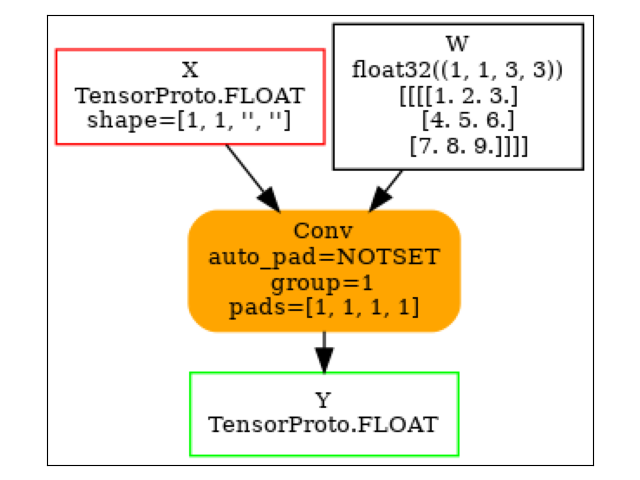
Execution

ref = ReferenceEvaluator(model)
ref.run(None, {"X": data[np.newaxis, np.newaxis, ...]})[0]

array([[[[ 134.,  211.,  250.,  289.,  328.,  367.,  238.],
         [ 333.,  492.,  537.,  582.,  627.,  672.,  423.],
         [ 564.,  807.,  852.,  897.,  942.,  987.,  612.],
         [ 795., 1122., 1167., 1212., 1257., 1302.,  801.],
         [ 422.,  571.,  592.,  613.,  634.,  655.,  382.]]]],
      dtype=float32)

Gradient

grad = onnx_derivative(
    model, options=DerivativeOptions.FillGrad | DerivativeOptions.KeepOutputs, verbose=1
)
plot_dot(grad)

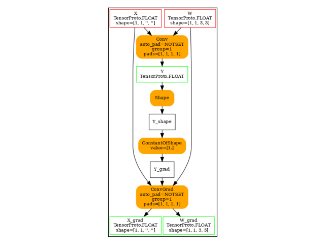
[_onnx_derivative_fw] weights=None inputs=None options=6
[_onnx_derivative_fw] guessed weights=['W']
[_onnx_derivative_fw] OrtModuleGraphBuilder
[_onnx_derivative_fw] TrainingGraphTransformerConfiguration with inputs_name=['X']
[_onnx_derivative_fw] builder initialize
[_onnx_derivative_fw] build
[_onnx_derivative_fw] final graph
[_onnx_derivative_fw] optimize
[_onnx_derivative_fw] done

<Axes: >

Execution.

sess = InferenceSession(grad.SerializeToString(), providers=["CPUExecutionProvider"])
res = sess.run(
    None,
    {
        "X": data[np.newaxis, np.newaxis, ...],
        "W": kernel[np.newaxis, np.newaxis, ...],
    },
)
res

[array([[[[12., 21., 21., 21., 21., 21., 16.],
         [27., 45., 45., 45., 45., 45., 33.],
         [27., 45., 45., 45., 45., 45., 33.],
         [27., 45., 45., 45., 45., 45., 33.],
         [24., 39., 39., 39., 39., 39., 28.]]]], dtype=float32), array([[[[312., 378., 336.],
         [495., 595., 525.],
         [480., 574., 504.]]]], dtype=float32), array([[[[ 134.,  211.,  250.,  289.,  328.,  367.,  238.],
         [ 333.,  492.,  537.,  582.,  627.,  672.,  423.],
         [ 564.,  807.,  852.,  897.,  942.,  987.,  612.],
         [ 795., 1122., 1167., 1212., 1257., 1302.,  801.],
         [ 422.,  571.,  592.,  613.,  634.,  655.,  382.]]]],
      dtype=float32)]

ConvTranspose

model = (
    start(ir_version=9, opset=18)
    .vin("X", shape=[1, 1, None, None])
    .cst(kernel[np.newaxis, np.newaxis, ...])
    .rename("W")
    .bring("X", "W")
    .ConvTranspose(pads=[1, 1, 1, 1])
    .rename("Y")
    .vout()
    .to_onnx()
)
plot_dot(model)

<Axes: >

Execution.

sess = InferenceSession(model.SerializeToString(), providers=["CPUExecutionProvider"])
ct = sess.run(None, {"X": impl[np.newaxis, np.newaxis, ...]})[0]
ct

array([[[[ 2672.,  5379.,  6804.,  7659.,  8514.,  8403.,  6254.],
         [ 8117., 15408., 18909., 20790., 22671., 21780., 15539.],
         [14868., 27315., 32400., 34425., 36450., 34191., 23922.],
         [20039., 35544., 41283., 43164., 45045., 41508., 28325.],
         [18608., 32055., 36756., 38151., 39546., 35943., 23966.]]]],
      dtype=float32)

im2col and col2im

Function im2col transforms an image so that the convolution of this image can be expressed as a matrix multiplication. It takes the image and the kernel shape.

def _get_indices(i: int, shape: Sequence[int]) -> np.array:
    res = np.empty((len(shape),), dtype=np.int64)
    k = len(shape) - 1
    while k > 0:
        m = i % shape[k]
        res[k] = m
        i -= m
        i /= shape[k]
        k -= 1
    res[0] = i
    return res


def _is_out(ind: Sequence[int], shape: Sequence[int]) -> bool:
    for i, s in zip(ind, shape):
        if i < 0:
            return True
        if i >= s:
            return True
    return False


def im2col_naive_implementation(
    data: np.array, kernel_shape: Sequence[int], fill_value: int = 0
) -> np.array:
    """
    Naive implementation for `im2col` or
    :func:`torch.nn.Unfold` (but with `padding=1`).

    :param image: image (float)
    :param kernel_shape: kernel shape
    :param fill_value: fill value
    :return: result
    """
    if not isinstance(kernel_shape, tuple):
        raise TypeError(f"Unexpected type {type(kernel_shape)!r} for kernel_shape.")
    if len(data.shape) != len(kernel_shape):
        raise ValueError(f"Shape mismatch {data.shape!r} and {kernel_shape!r}.")
    output_shape = data.shape + kernel_shape
    res = np.empty(output_shape, dtype=data.dtype)
    middle = np.array([-m / 2 for m in kernel_shape], dtype=np.int64)
    kernel_size = np.prod(kernel_shape)
    data_size = np.prod(data.shape)
    for i in range(data_size):
        for j in range(kernel_size):
            i_data = _get_indices(i, data.shape)
            i_kernel = _get_indices(j, kernel_shape)
            ind = i_data + i_kernel + middle
            t_data = tuple(i_data)
            t_kernel = tuple(i_kernel)
            i_out = t_data + t_kernel
            res[i_out] = fill_value if _is_out(ind, data.shape) else data[tuple(ind)]
    return res


v = np.arange(5).astype(np.float32)
w = im2col_naive_implementation(v, (3,))
w

array([[0., 0., 1.],
       [0., 1., 2.],
       [1., 2., 3.],
       [2., 3., 4.],
       [3., 4., 0.]], dtype=float32)

All is left is the matrix multiplication.

k = np.array([1, 1, 1], dtype=np.float32)
conv = w @ k
conv

array([1., 3., 6., 9., 7.], dtype=float32)

Let’s compare with the numpy function.

np.convolve(v, k, mode="same")

array([1., 3., 6., 9., 7.], dtype=float32)

..math:

conv(v, k) = im2col(v, shape(k)) \; k = w \; k` where `w = im2col(v, shape(k))

In deep neural network, the gradient is propagated from the last layer to the first one. At some point, the backpropagation produces the gradient , the gradient of the error against the outputs of the convolution layer. Then .

We need to compute .

We can say that .

That leaves . And this last term is equal to where is a matrix identical to except that all not null parameter are replaced by 1. To summarize: .

Finally:

Now, is a very simple matrix with only ones or zeros. Is there a way we can avoid doing the matrix multiplication but simply adding terms? That’s the purpose of function col2im defined so that: