Tree-Ensemble Statistics#

stats_tree_ensemble() computes per-tree and per-feature statistics for TreeEnsembleClassifier and TreeEnsembleRegressor ONNX nodes (from the ai.onnx.ml domain).

The function returns a NodeStatistics instance containing:

global counts — number of trees, features, outputs, split modes, …
per-feature threshold distributions (HistTreeStatistics)
per-tree structure summaries (TreeStatistics)

enumerate_stats_nodes() walks a full ModelProto and yields statistics for every matching node in one call, which is convenient for exploring real-world models built from scikit-learn RandomForestClassifier or similar estimators.

1. Train a scikit-learn RandomForestClassifier on dummy data#

We generate a small binary-classification dataset with four features and train a five-tree random forest with depth ≤ 4.

import numpy as np
from sklearn.ensemble import RandomForestClassifier

rng = np.random.default_rng(0)
X_train = rng.standard_normal((200, 4)).astype(np.float32)
y_train = (X_train[:, 0] + X_train[:, 2] > 0).astype(int)

clf = RandomForestClassifier(n_estimators=5, max_depth=4, random_state=0)
clf.fit(X_train, y_train)
print(
    f"Trained RandomForestClassifier: {clf.n_estimators} trees, "
    f"{clf.n_features_in_} features, classes={list(clf.classes_)}"
)

Trained RandomForestClassifier: 5 trees, 4 features, classes=[np.int64(0), np.int64(1)]

2. Convert to ONNX with yobx.sklearn.to_onnx#

yobx.sklearn.to_onnx() converts the estimator and returns an ExportArtifact. The .proto attribute gives the ModelProto containing a TreeEnsembleClassifier node in the ai.onnx.ml domain — the operator supported by stats_tree_ensemble().

from yobx.sklearn import to_onnx  # noqa: E402

artifact = to_onnx(clf, (X_train,), target_opset={"": 20, "ai.onnx.ml": 3})
model = artifact.proto

print("Graph nodes:", [(n.op_type, n.domain) for n in model.graph.node])

Graph nodes: [('TreeEnsembleClassifier', 'ai.onnx.ml')]

3. Compute statistics for the tree-ensemble node#

enumerate_stats_nodes() walks the model graph and returns a NodeStatistics for every TreeEnsembleClassifier / TreeEnsembleRegressor it encounters.

from yobx.helpers import enumerate_stats_nodes  # noqa: E402

# Collect results from the full model walk
all_stats = list(enumerate_stats_nodes(model))
print(f"\nNumber of tree-ensemble nodes found: {len(all_stats)}")

# For the single classifier node, inspect the statistics directly
_path, _parent, stats = all_stats[0]
print("kind      :", stats["kind"])
print("n_trees   :", stats["n_trees"])
print("n_outputs :", stats["n_outputs"])
print("n_features:", stats["n_features"])
print("n_rules   :", stats["n_rules"])
print("rules     :", stats["rules"])
print("hist_rules:", stats["hist_rules"])

Number of tree-ensemble nodes found: 1
kind      : Classifier
n_trees   : 5
n_outputs : 2
n_features: 4
n_rules   : 2
rules     : {np.str_('LEAF'), np.str_('BRANCH_LEQ')}
hist_rules: Counter({np.str_('LEAF'): 54, np.str_('BRANCH_LEQ'): 49})

4. Per-tree breakdown#

The "trees" key holds a TreeStatistics object for each tree in the ensemble.

print(f"\nPer-tree statistics ({stats['n_trees']} trees):")
for tr in stats["trees"]:
    row = tr.dict_values
    print(
        f"  tree {tr.tree_id}:"
        f" n_nodes={row['n_nodes']}"
        f" n_leaves={row['n_leaves']}"
        f" n_features={row['n_features']}"
    )

Per-tree statistics (5 trees):
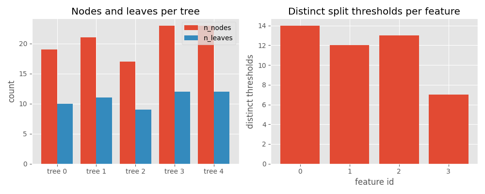
  tree 0: n_nodes=19 n_leaves=10 n_features=3
  tree 1: n_nodes=21 n_leaves=11 n_features=4
  tree 2: n_nodes=17 n_leaves=9 n_features=3
  tree 3: n_nodes=23 n_leaves=12 n_features=3
  tree 4: n_nodes=23 n_leaves=12 n_features=4

5. Per-feature threshold distribution#

For each input feature that appears as a split condition, HistTreeStatistics stores the distribution of threshold values used across all trees.

print(f"\nPer-feature threshold statistics ({len(stats['features'])} features):")
for feat in stats["features"]:
    row = feat.dict_values
    print(
        f"  feature {feat.featureid}:"
        f" min={row['min']:.3f}"
        f" max={row['max']:.3f}"
        f" mean={row['mean']:.3f}"
        f" n_distinct={row['n_distinct']}"
    )

Per-feature threshold statistics (4 features):
  feature 0: min=-1.268 max=1.492 mean=0.025 n_distinct=14
  feature 1: min=-0.942 max=1.756 mean=0.597 n_distinct=12
  feature 2: min=-1.702 max=1.192 mean=-0.052 n_distinct=13
  feature 3: min=-1.688 max=2.250 mean=0.374 n_distinct=7

6. Flat dictionary for DataFrame integration#

dict_values() flattens all scalar statistics into a single dict suitable for creating a pandas DataFrame row.

row = stats.dict_values
print("\nFlat stats dict:")
for k, v in sorted(row.items()):
    print(f"  {k}: {v}")

Flat stats dict:
  hist_rules__BRANCH_LEQ: 49
  hist_rules__LEAF: 54
  kind: Classifier
  max_featureid: 3
  n_features: 4
  n_outputs: 2
  n_rules: 2
  n_trees: 5
  rules: BRANCH_LEQ,LEAF

7. Visualize tree statistics with matplotlib#

Plot per-tree node/leaf counts and per-feature split counts side by side.

import matplotlib.pyplot as plt  # noqa: E402

fig, (ax1, ax2) = plt.subplots(1, 2, figsize=(10, 4))

# --- left panel: nodes and leaves per tree ---
tree_ids = [tr.tree_id for tr in stats["trees"]]
n_nodes = [tr["n_nodes"] for tr in stats["trees"]]
n_leaves = [tr["n_leaves"] for tr in stats["trees"]]
x = range(len(tree_ids))
ax1.bar([i - 0.2 for i in x], n_nodes, width=0.4, label="n_nodes")
ax1.bar([i + 0.2 for i in x], n_leaves, width=0.4, label="n_leaves")
ax1.set_xticks(list(x))
ax1.set_xticklabels([f"tree {t}" for t in tree_ids])
ax1.set_ylabel("count")
ax1.set_title("Nodes and leaves per tree")
ax1.legend()

# --- right panel: number of split thresholds per feature ---
feat_ids = [f.featureid for f in stats["features"]]
n_splits = [f["n_distinct"] for f in stats["features"]]
ax2.bar(feat_ids, n_splits)
ax2.set_xlabel("feature id")
ax2.set_ylabel("distinct thresholds")
ax2.set_title("Distinct split thresholds per feature")
ax2.set_xticks(feat_ids)

fig.tight_layout()
plt.show()