Symbolic Cost of a Model: Attention Block#

This example shows how to compute the symbolic FLOPs cost of an ONNX model using BasicShapeBuilder with inference=InferenceMode.COST.

The model used is a single-head scaled dot-product attention block, which contains two MatMul nodes (the core of the attention mechanism) plus auxiliary element-wise operations.

We also show how a simple pattern-based optimization can reduce the total number of floating-point operations. Specifically, the MulMulMatMulPattern fuses

Mul(Q, scale_q)  ──┐
                   MatMul  →  Mul(MatMul(Q, Kᵀ), scale_q * scale_k)
Mul(Kᵀ, scale_k) ──┘

removing the two element-wise multiplications on the larger (batch, seq, d_head) tensors and replacing them with a single multiplication on the smaller (batch, seq, seq) score tensor.

import numpy as np
import onnx
import onnx.helper as oh
import onnx.numpy_helper as onh

from yobx.xbuilder import GraphBuilder, OptimizationOptions
from yobx.xshape import BasicShapeBuilder, InferenceMode

TFLOAT = onnx.TensorProto.FLOAT

1. Build the attention model#

The graph implements scaled dot-product attention:

$\text{out} = \text{Softmax}(Q \cdot s_Q \cdot (K^T \cdot s_K)) \cdot V$

where scale_q = 1 / sqrt(d_head) and scale_k = 1.0. Both inputs to the attention MatMul are multiplied by a constant scalar, which creates an opportunity for the MulMulMatMulPattern to fuse them.

Input dimensions are symbolic (batch, seq, d_head) so that the cost expressions remain general.

scale_q = np.array([0.125], dtype=np.float32)  # 1 / sqrt(64)
scale_k = np.array([1.0], dtype=np.float32)

model = oh.make_model(
    oh.make_graph(
        [
            # Scale Q by a constant factor (1 / sqrt(d_head))
            oh.make_node("Mul", ["Q", "scale_q"], ["Q_scaled"]),
            # Transpose K: (batch, seq, d_head) → (batch, d_head, seq)
            oh.make_node("Transpose", ["K"], ["K_T"], perm=[0, 2, 1]),
            # Scale K_T by a second constant factor
            oh.make_node("Mul", ["K_T", "scale_k"], ["K_T_scaled"]),
            # Attention scores: (batch, seq, d_head) × (batch, d_head, seq) → (batch, seq, seq)
            oh.make_node("MatMul", ["Q_scaled", "K_T_scaled"], ["scores"]),
            # Softmax over the last axis
            oh.make_node("Softmax", ["scores"], ["attn_weights"], axis=-1),
            # Weighted sum of values: (batch, seq, seq) × (batch, seq, d_head)
            oh.make_node("MatMul", ["attn_weights", "V"], ["output"]),
        ],
        "sdp_attention",
        [
            oh.make_tensor_value_info("Q", TFLOAT, ["batch", "seq", "d_head"]),
            oh.make_tensor_value_info("K", TFLOAT, ["batch", "seq", "d_head"]),
            oh.make_tensor_value_info("V", TFLOAT, ["batch", "seq", "d_head"]),
        ],
        [oh.make_tensor_value_info("output", TFLOAT, None)],
        [onh.from_array(scale_q, name="scale_q"), onh.from_array(scale_k, name="scale_k")],
    ),
    opset_imports=[oh.make_opsetid("", 18)],
    ir_version=10,
)

print("Nodes in the original model:")
for node in model.graph.node:
    print(f"  {node.op_type:12s}  inputs={list(node.input)}  outputs={list(node.output)}")

Nodes in the original model:
  Mul           inputs=['Q', 'scale_q']  outputs=['Q_scaled']
  Transpose     inputs=['K']  outputs=['K_T']
  Mul           inputs=['K_T', 'scale_k']  outputs=['K_T_scaled']
  MatMul        inputs=['Q_scaled', 'K_T_scaled']  outputs=['scores']
  Softmax       inputs=['scores']  outputs=['attn_weights']
  MatMul        inputs=['attn_weights', 'V']  outputs=['output']

2. Compute the symbolic cost#

BasicShapeBuilder.run_model() with inference=InferenceMode.COST walks every node and calls estimate_node_flops() on each one. Because the model inputs have symbolic dimensions, the returned FLOPs values are symbolic arithmetic expressions (strings such as "2*batch*d_head*seq*seq").

Transpose costs 1 read + 1 write per element (input element count). Truly zero-cost ops (Reshape, Identity, Cast, …) return 0.

builder_before = BasicShapeBuilder()
cost_before = builder_before.run_model(model, inference=InferenceMode.COST)

print("Symbolic FLOPs per node (before optimization):")
for op_type, flops, _ in cost_before:
    if flops:
        print(f"  {op_type:12s}  {flops}")

Symbolic FLOPs per node (before optimization):
  Mul           batch*d_head*seq
  Transpose     batch*d_head*seq
  Mul           batch*d_head*seq
  MatMul        2*batch*d_head*seq*seq
  Softmax       3*batch*seq*seq
  MatMul        2*batch*d_head*seq*seq

3. Evaluate the symbolic FLOPs with concrete input shapes#

Once we have actual input tensors, evaluate_cost_with_true_inputs() substitutes the true dimension values into every symbolic expression and returns concrete integer FLOPs.

batch, seq, d_head = 2, 64, 64
rng = np.random.default_rng(42)
feeds = {
    "Q": rng.standard_normal((batch, seq, d_head)).astype(np.float32),
    "K": rng.standard_normal((batch, seq, d_head)).astype(np.float32),
    "V": rng.standard_normal((batch, seq, d_head)).astype(np.float32),
}

cost_concrete_before = builder_before.evaluate_cost_with_true_inputs(feeds, cost_before)

print("Concrete FLOPs per node (before optimization):")
total_before = 0
for op_type, flops, _ in cost_concrete_before:
    total_before += flops or 0
    if flops:
        print(f"  {op_type:12s}  {flops:>10,}")
print(f"  {'TOTAL':12s}  {total_before:>10,}")

Concrete FLOPs per node (before optimization):
  Mul                8,192
  Transpose          8,192
  Mul                8,192
  MatMul         1,048,576
  Softmax           24,576
  MatMul         1,048,576
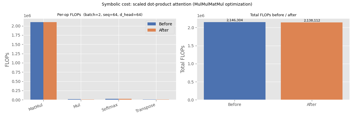
  TOTAL          2,146,304

4. Apply the MulMulMatMulPattern optimization#

The MulMulMatMulPattern detects a MatMul whose both inputs are the outputs of element-wise Mul nodes with constant scalars. It fuses the three nodes into a single MatMul followed by one Mul on the output tensor.

For our attention model this turns:

Mul(Q, scale_q) on a (batch, seq, d_head) tensor — removed
Mul(K_T, scale_k) on a (batch, d_head, seq) tensor — removed
MatMul(Q_scaled, K_T_scaled)

into:

MatMul(Q, K_T)
Mul(scores, scale_q * scale_k) on a (batch, seq, seq) tensor — new, smaller

gr = GraphBuilder(
    model,
    infer_shapes_options=True,
    optimization_options=OptimizationOptions(patterns=["MulMulMatMul"], verbose=0),
)
opt_artifact = gr.to_onnx(optimize=True)
opt_model = opt_artifact.proto  # ExportArtifact wraps a ModelProto

print("Nodes in the optimized model:")
for node in opt_model.graph.node:
    print(f"  {node.op_type:12s}  inputs={list(node.input)}  outputs={list(node.output)}")

Nodes in the optimized model:
  Transpose     inputs=['K']  outputs=['K_T']
  MatMul        inputs=['Q', 'K_T']  outputs=['MulMulMatMulPattern_scores']
  Mul           inputs=['MulMulMatMulPattern_scores', 'scale_q']  outputs=['scores']
  Softmax       inputs=['scores']  outputs=['attn_weights']
  MatMul        inputs=['attn_weights', 'V']  outputs=['output']

5. Compute the symbolic cost of the optimized model#

We run the same symbolic cost analysis on the optimized model.

builder_after = BasicShapeBuilder()
cost_after = builder_after.run_model(opt_model, inference=InferenceMode.COST)

print("Symbolic FLOPs per node (after optimization):")
for op_type, flops, _ in cost_after:
    if flops:
        print(f"  {op_type:12s}  {flops}")

Symbolic FLOPs per node (after optimization):
  Transpose     batch*d_head*seq
  MatMul        2*batch*d_head*seq*seq
  Mul           batch*seq*seq
  Softmax       3*batch*seq*seq
  MatMul        2*batch*d_head*seq*seq

6. Evaluate the optimized model with concrete shapes#

The same feeds dictionary is used so that the results are directly comparable.

cost_concrete_after = builder_after.evaluate_cost_with_true_inputs(feeds, cost_after)

print("Concrete FLOPs per node (after optimization):")
total_after = 0
for op_type, flops, _ in cost_concrete_after:
    total_after += flops or 0
    if flops:
        print(f"  {op_type:12s}  {flops:>10,}")
print(f"  {'TOTAL':12s}  {total_after:>10,}")
print(
    f"\nFLOPs saved: {total_before - total_after:,}  "
    f"({(total_before - total_after) / total_before:.2%})"
)

Concrete FLOPs per node (after optimization):
  Transpose          8,192
  MatMul         1,048,576
  Mul                8,192
  Softmax           24,576
  MatMul         1,048,576
  TOTAL          2,138,112

FLOPs saved: 8,192  (0.38%)

7. Visualise the comparison#

The bar chart below groups operations by type and shows the FLOPs contribution before and after the optimization.

MatMul (and Softmax) FLOPs are unchanged — only the surrounding Mul operations are affected.
The two large Mul nodes on (batch, seq, d_head) tensors are replaced by one smaller Mul on the (batch, seq, seq) score tensor, saving batch * seq * (2 * d_head − seq) FLOPs in total.

import matplotlib.pyplot as plt  # noqa: E402


# Aggregate FLOPs by op type
def _aggregate(cost_list):
    totals = {}
    for op_type, flops, _ in cost_list:
        totals[op_type] = totals.get(op_type, 0) + (flops or 0)
    return totals


agg_before = _aggregate(cost_concrete_before)
agg_after = _aggregate(cost_concrete_after)

all_ops = sorted(op for op in set(agg_before) | set(agg_after))

vals_before = [agg_before.get(op, 0) for op in all_ops]
vals_after = [agg_after.get(op, 0) for op in all_ops]

x = np.arange(len(all_ops))
width = 0.35

fig, axes = plt.subplots(1, 2, figsize=(12, 4))

# Left: per-op FLOPs
ax = axes[0]
bars_b = ax.bar(x - width / 2, vals_before, width, label="Before", color="#4c72b0")
bars_a = ax.bar(x + width / 2, vals_after, width, label="After", color="#dd8452")
ax.set_xticks(x)
ax.set_xticklabels(all_ops, rotation=20, ha="right")
ax.set_ylabel("FLOPs")
ax.set_title(f"Per-op FLOPs  (batch={batch}, seq={seq}, d_head={d_head})", fontsize=9)
ax.legend()

# Right: total FLOPs bar
ax2 = axes[1]
bars_total = ax2.bar(
    ["Before", "After"], [total_before, total_after], color=["#4c72b0", "#dd8452"]
)
ax2.set_ylabel("Total FLOPs")
ax2.set_title("Total FLOPs before / after", fontsize=9)
for bar, val in zip(bars_total, [total_before, total_after]):
    ax2.text(
        bar.get_x() + bar.get_width() / 2,
        bar.get_height() * 1.005,
        f"{val:,}",
        ha="center",
        va="bottom",
        fontsize=8,
    )

plt.suptitle(
    "Symbolic cost: scaled dot-product attention (MulMulMatMul optimization)", fontsize=10
)
plt.tight_layout()
plt.show()