Note
Go to the end to download the full example code.
Command Line: python -m yobx print#
This example builds a small ONNX model, saves it to a temporary file, and
then demonstrates the different output formats produced by the
python -m yobx print command.
The same result can be achieved from the terminal with:
import os
import tempfile
import onnx
import onnx.helper as oh
from yobx._command_lines_parser import _cmd_print

TFLOAT = onnx.TensorProto.FLOAT
Build a small ONNX model#
The graph computes Z = Relu(X + Y) with static shapes (2, 3).
model = oh.make_model(
    oh.make_graph(
        [oh.make_node("Add", ["X", "Y"], ["added"]), oh.make_node("Relu", ["added"], ["Z"])],
        "add_relu",
        [
            oh.make_tensor_value_info("X", TFLOAT, [2, 3]),
            oh.make_tensor_value_info("Y", TFLOAT, [2, 3]),
        ],
        [oh.make_tensor_value_info("Z", TFLOAT, [2, 3])],
    ),
    opset_imports=[oh.make_opsetid("", 18)],
    ir_version=10,
)

# Save to a temporary file so the CLI helpers can load it.
fd, tmp = tempfile.mkstemp(suffix=".onnx")
os.close(fd)
onnx.save(model, tmp)
pretty format#
The default format produced by
yobx.helpers.onnx_helper.pretty_onnx().
It shows opset, inputs/outputs, and every node in a compact,
human-readable layout.
print("python -m yobx print pretty model.onnx")
print("-" * 40)
_cmd_print(["print", "pretty", tmp])
python -m yobx print pretty model.onnx
----------------------------------------
opset: domain='' version=18
input: name='X' type=dtype('float32') shape=[2, 3]
input: name='Y' type=dtype('float32') shape=[2, 3]
Add(X, Y) -> added
  Relu(added) -> Z
output: name='Z' type=dtype('float32') shape=[2, 3]
printer format#
Uses the built-in onnx.printer.to_text renderer which produces the
official ONNX text representation.
print("python -m yobx print printer model.onnx")
print("-" * 40)
_cmd_print(["print", "printer", tmp])
python -m yobx print printer model.onnx
----------------------------------------
<
   ir_version: 10,
   opset_import: ["" : 18]
>
add_relu (float[2,3] X, float[2,3] Y) => (float[2,3] Z) {
   added = Add (X, Y)
   Z = Relu (added)
}
dot format#
Dumps the DOT graph source. Pipe the output to dot -Tsvg to get
a visual representation of the graph
(see also yobx.helpers.dot_helper.to_dot()).
print("python -m yobx print dot model.onnx")
print("-" * 40)
_cmd_print(["print", "dot", tmp])
python -m yobx print dot model.onnx
----------------------------------------
digraph {
  graph [rankdir=TB, splines=true, overlap=false, nodesep=0.2, ranksep=0.2, fontsize=8];
  node [style="rounded,filled", color="#888888", fontcolor="#222222", shape=box];
  edge [arrowhead=vee, fontsize=7, labeldistance=-5, labelangle=0];
  I_0 [label="X\nFLOAT(2,3)", fillcolor="#aaeeaa"];
  I_1 [label="Y\nFLOAT(2,3)", fillcolor="#aaeeaa"];
  Add_2 [label="Add(., .)", fillcolor="#cccccc"];
  Relu_3 [label="Relu(.)", fillcolor="#cccccc"];
  I_0 -> Add_2 [label="FLOAT(2,3)"];
  I_1 -> Add_2 [label="FLOAT(2,3)"];
  Add_2 -> Relu_3 [label="FLOAT(2,3)"];
  O_4 [label="Z\nFLOAT(2,3)", fillcolor="#aaaaee"];
  Relu_3 -> O_4;
}
mermaid format#
Dumps a Mermaid flowchart TD diagram.
Paste the output into the Mermaid live editor or any Markdown renderer that
supports Mermaid fenced code blocks to get an interactive graph visualisation
(see also yobx.translate.mermaid_emitter.MermaidEmitter).
print("python -m yobx print mermaid model.onnx")
print("-" * 40)
_cmd_print(["print", "mermaid", tmp])
python -m yobx print mermaid model.onnx
----------------------------------------
flowchart TD
    I_0["X\nFLOAT(2,3)"]:::input
    I_1["Y\nFLOAT(2,3)"]:::input
    Add_2["Add(., .)"]:::op
    Relu_3["Relu(.)"]:::op
    I_0 -->|"FLOAT(2,3)"| Add_2
    I_1 -->|"FLOAT(2,3)"| Add_2
    Add_2 --> Relu_3
    O_4["Z\nFLOAT(2,3)"]:::output
    Relu_3 --> O_4
    classDef input fill:#aaeeaa,stroke:#00aa00,color:#000
    classDef init fill:#cccc00,stroke:#888800,color:#000
    classDef op fill:#cccccc,stroke:#666666,color:#000
    classDef output fill:#aaaaee,stroke:#0000aa,color:#000
Total running time of the script: (0 minutes 0.040 seconds)
Related examples

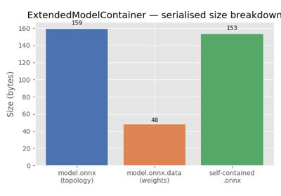
ExtendedModelContainer: large-initializer ONNX models