Random order for a sum

Parallelization usually means a summation is done with a random order. That may lead to different values if the computation is made many times even though the result should be the same. This example compares summation of random permutation of the same array of values.

Setup

from tqdm import tqdm
import numpy as np
import pandas

unique_values = np.array(
    [2.1102535724639893, 0.5986238718032837, -0.49545818567276], dtype=np.float32
)
random_index = np.random.randint(0, 3, 2000)
assert set(random_index) == {0, 1, 2}
values = unique_values[random_index]

s0 = values.sum()
s1 = np.array(0, dtype=np.float32)
for n in values:
    s1 += n

delta = s1 - s0
print(f"reduced sum={s0}, iterative sum={s1}, delta={delta}")

reduced sum=1469.287841796875, iterative sum=1469.273681640625, delta=-0.01416015625

There are discrepancies.

Random order

Let’s go further and check the sum of random permutation of the same set. Let’s compare the result with the same sum done with a higher precision (double).

def check_orders(values, n=200, bias=0):
    double_sums = []
    sums = []
    reduced_sums = []
    reduced_dsums = []
    for _i in tqdm(range(n)):
        permuted_values = np.random.permutation(values)
        s = np.array(bias, dtype=np.float32)
        sd = np.array(bias, dtype=np.float64)
        for n in permuted_values:
            s += n
            sd += n
        sums.append(s)
        double_sums.append(sd)
        reduced_sums.append(permuted_values.sum() + bias)
        reduced_dsums.append(permuted_values.astype(np.float64).sum() + bias)

    data = []
    mi, ma = min(sums), max(sums)
    data.append(dict(name="seq_fp32", min=mi, max=ma, bias=bias))
    print(f"min={mi} max={ma} delta={ma-mi}")
    mi, ma = min(double_sums), max(double_sums)
    data.append(dict(name="seq_fp64", min=mi, max=ma, bias=bias))
    print(f"min={mi} max={ma} delta={ma-mi} (double)")
    mi, ma = min(reduced_sums), max(reduced_sums)
    data.append(dict(name="red_f32", min=mi, max=ma, bias=bias))
    print(f"min={mi} max={ma} delta={ma-mi} (reduced)")
    mi, ma = min(reduced_dsums), max(reduced_dsums)
    data.append(dict(name="red_f64", min=mi, max=ma, bias=bias))
    print(f"min={mi} max={ma} delta={ma-mi} (reduced)")
    return data


data1 = check_orders(values)

  0%|          | 0/200 [00:00<?, ?it/s]
  8%|▊         | 17/200 [00:00<00:01, 157.95it/s]
 16%|█▋        | 33/200 [00:00<00:01, 158.56it/s]
 24%|██▍       | 49/200 [00:00<00:00, 156.65it/s]
 33%|███▎      | 66/200 [00:00<00:00, 160.35it/s]
 42%|████▏     | 84/200 [00:00<00:00, 166.65it/s]
 52%|█████▏    | 104/200 [00:00<00:00, 175.62it/s]
 62%|██████▏   | 124/200 [00:00<00:00, 181.88it/s]
 72%|███████▏  | 143/200 [00:00<00:00, 181.78it/s]
 81%|████████  | 162/200 [00:00<00:00, 180.87it/s]
 90%|█████████ | 181/200 [00:01<00:00, 171.88it/s]
100%|█████████▉| 199/200 [00:01<00:00, 159.86it/s]
100%|██████████| 200/200 [00:01<00:00, 167.60it/s]
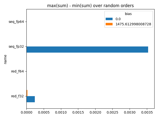
min=1469.271728515625 max=1469.2750244140625 delta=0.0032958984375
min=1469.2879551649094 max=1469.2879551649094 delta=0.0 (double)
min=1469.287841796875 max=1469.2879638671875 delta=0.0001220703125 (reduced)
min=1469.2879551649094 max=1469.2879551649094 delta=0.0 (reduced)

This example clearly shows the order has an impact. It is usually unavoidable but it could reduced if the sum it close to zero. In that case, the sum would be of the same order of magnitude of the add values.

Removing the average

Computing the average of the values requires to compute the sum. However if we have an estimator of this average, not necessarily the exact value, we would help the summation to keep the same order of magnitude than the values it adds.

mean = unique_values.mean()
values -= mean
data2 = check_orders(values, bias=len(values) * mean)

  0%|          | 0/200 [00:00<?, ?it/s]
  8%|▊         | 16/200 [00:00<00:01, 149.59it/s]
 16%|█▌        | 31/200 [00:00<00:01, 128.28it/s]
 25%|██▌       | 50/200 [00:00<00:00, 151.50it/s]
 33%|███▎      | 66/200 [00:00<00:00, 137.13it/s]
 42%|████▏     | 83/200 [00:00<00:00, 143.54it/s]
 49%|████▉     | 98/200 [00:00<00:00, 138.97it/s]
 56%|█████▋    | 113/200 [00:00<00:00, 134.49it/s]
 66%|██████▌   | 132/200 [00:00<00:00, 146.07it/s]
 74%|███████▍  | 148/200 [00:01<00:00, 148.20it/s]
 82%|████████▏ | 163/200 [00:01<00:00, 147.88it/s]
 90%|█████████ | 180/200 [00:01<00:00, 154.09it/s]
100%|█████████▉| 199/200 [00:01<00:00, 162.71it/s]
100%|██████████| 200/200 [00:01<00:00, 148.76it/s]
min=1469.288330078125 max=1469.288330078125 delta=0.0
min=1469.2879548072815 max=1469.2879548072815 delta=0.0 (double)
min=1469.2879638671875 max=1469.2879638671875 delta=0.0 (reduced)
min=1469.2879548072815 max=1469.2879548072815 delta=0.0 (reduced)

The differences are clearly lower.

df = pandas.DataFrame(data1 + data2)
df["delta"] = df["max"] - df["min"]
piv = df.pivot(index="name", columns="bias", values="delta")
print(piv)

bias     0.000000    1475.613037
name
red_f32     0.000122         0.0
red_f64          0.0         0.0
seq_fp32    0.003296         0.0
seq_fp64         0.0         0.0

Plots.

ax = piv.plot.barh()
ax.set_title("max(sum) - min(sum) over random orders")
ax.get_figure().tight_layout()
ax.get_figure().savefig("plot_check_random_order.png")