Note
Go to the end to download the full example code.
Compares matrix multiplication implementations
numpy has a very fast implementation of matrix multiplication. There are many ways to be slower.
Compared implementations:
import pprint
import numpy
from numpy.testing import assert_almost_equal
import matplotlib.pyplot as plt
from pandas import DataFrame, concat
from teachcompute.validation.cython.mul_cython_omp import dmul_cython_omp
from teachcompute.ext_test_case import measure_time_dim, unit_test_going

dfs = []
if unit_test_going():
    sets = [2, 4, 6]
else:
    sets = list(range(2, 145, 20))
numpy mul
ctxs = [
    dict(
        va=numpy.random.randn(n, n).astype(numpy.float64),
        vb=numpy.random.randn(n, n).astype(numpy.float64),
        mul=lambda x, y: x @ y,
        x_name=n,
    )
    for n in sets
]

res = list(measure_time_dim("mul(va, vb)", ctxs, verbose=1))
dfs.append(DataFrame(res))
dfs[-1]["fct"] = "numpy"
pprint.pprint(dfs[-1].tail(n=2))
  0%|          | 0/8 [00:00<?, ?it/s]
100%|██████████| 8/8 [00:00<00:00, 45.89it/s]
100%|██████████| 8/8 [00:00<00:00, 45.79it/s]
    average  deviation  min_exec  max_exec  repeat  number     ttime  context_size  warmup_time  x_name    fct
6  0.000068   0.000010  0.000057  0.000091      10      50  0.000677           184     0.000330     122  numpy
7  0.000148   0.000019  0.000124  0.000176      10      50  0.001481           184     0.000509     142  numpy
Simple multiplication
ctxs = [
    dict(
        va=numpy.random.randn(n, n).astype(numpy.float64),
        vb=numpy.random.randn(n, n).astype(numpy.float64),
        mul=dmul_cython_omp,
        x_name=n,
    )
    for n in sets
]

res = list(measure_time_dim("mul(va, vb)", ctxs, verbose=1))
pprint.pprint(res[-1])
  0%|          | 0/8 [00:00<?, ?it/s]
 50%|█████     | 4/8 [00:00<00:00, 26.29it/s]
 88%|████████▊ | 7/8 [00:01<00:00,  4.46it/s]
100%|██████████| 8/8 [00:02<00:00,  3.29it/s]
{'average': np.float64(0.002170637821996934),
 'context_size': 184,
 'deviation': np.float64(0.00016493075762814832),
 'max_exec': np.float64(0.0023841295799866204),
 'min_exec': np.float64(0.0018377313399832928),
 'number': 50,
 'repeat': 10,
 'ttime': np.float64(0.02170637821996934),
 'warmup_time': 0.0017737540001689922,
 'x_name': 142}
Other scenarios
3 differents algorithms, each of them parallelized.
See dmul_cython_omp.
for algo in range(2):
    for parallel in (0, 1):
        print("algo=%d parallel=%d" % (algo, parallel))
        ctxs = [
            dict(
                va=numpy.random.randn(n, n).astype(numpy.float64),
                vb=numpy.random.randn(n, n).astype(numpy.float64),
                mul=lambda x, y, algo=algo, parallel=parallel: dmul_cython_omp(
                    x, y, algo=algo, parallel=parallel
                ),
                x_name=n,
            )
            for n in sets
        ]

        res = list(measure_time_dim("mul(va, vb)", ctxs, verbose=1))
        dfs.append(DataFrame(res))
        dfs[-1]["fct"] = "a=%d-p=%d" % (algo, parallel)
        pprint.pprint(dfs[-1].tail(n=2))
algo=0 parallel=0

  0%|          | 0/8 [00:00<?, ?it/s]
 50%|█████     | 4/8 [00:00<00:00, 29.62it/s]
 88%|████████▊ | 7/8 [00:01<00:00,  4.60it/s]
100%|██████████| 8/8 [00:02<00:00,  3.41it/s]
    average  deviation  min_exec  max_exec  repeat  number     ttime  context_size  warmup_time  x_name      fct
6  0.001293   0.000107  0.001110  0.001480      10      50  0.012928           184     0.001114     122  a=0-p=0
7  0.002087   0.000114  0.001895  0.002272      10      50  0.020871           184     0.001809     142  a=0-p=0
algo=0 parallel=1

  0%|          | 0/8 [00:00<?, ?it/s]
 12%|█▎        | 1/8 [00:00<00:03,  2.13it/s]
 25%|██▌       | 2/8 [00:00<00:02,  2.20it/s]
 38%|███▊      | 3/8 [00:01<00:02,  2.28it/s]
 50%|█████     | 4/8 [00:01<00:01,  2.24it/s]
 62%|██████▎   | 5/8 [00:02<00:01,  2.19it/s]
 75%|███████▌  | 6/8 [00:02<00:00,  2.08it/s]
 88%|████████▊ | 7/8 [00:03<00:00,  1.89it/s]
100%|██████████| 8/8 [00:04<00:00,  1.74it/s]
100%|██████████| 8/8 [00:04<00:00,  1.96it/s]
    average  deviation  min_exec  max_exec  repeat  number     ttime  context_size  warmup_time  x_name      fct
6  0.001251   0.000110  0.001084  0.001488      10      50  0.012507           184     0.002039     122  a=0-p=1
7  0.001331   0.000075  0.001209  0.001458      10      50  0.013310           184     0.001823     142  a=0-p=1
algo=1 parallel=0

  0%|          | 0/8 [00:00<?, ?it/s]
 50%|█████     | 4/8 [00:00<00:00, 39.45it/s]
100%|██████████| 8/8 [00:02<00:00,  3.10it/s]
100%|██████████| 8/8 [00:02<00:00,  3.59it/s]
    average  deviation  min_exec  max_exec  repeat  number     ttime  context_size  warmup_time  x_name      fct
6  0.001231   0.000136  0.001039  0.001492      10      50  0.012310           184     0.001038     122  a=1-p=0
7  0.002045   0.000129  0.001813  0.002221      10      50  0.020447           184     0.001809     142  a=1-p=0
algo=1 parallel=1

  0%|          | 0/8 [00:00<?, ?it/s]
 12%|█▎        | 1/8 [00:00<00:02,  2.39it/s]
 25%|██▌       | 2/8 [00:00<00:02,  2.43it/s]
 38%|███▊      | 3/8 [00:01<00:02,  2.37it/s]
 50%|█████     | 4/8 [00:01<00:01,  2.41it/s]
 62%|██████▎   | 5/8 [00:02<00:01,  2.39it/s]
 75%|███████▌  | 6/8 [00:02<00:00,  2.26it/s]
 88%|████████▊ | 7/8 [00:03<00:00,  2.05it/s]
100%|██████████| 8/8 [00:03<00:00,  1.79it/s]
100%|██████████| 8/8 [00:03<00:00,  2.07it/s]
    average  deviation  min_exec  max_exec  repeat  number     ttime  context_size  warmup_time  x_name      fct
6  0.001157   0.000115  0.000982  0.001342      10      50  0.011568           184     0.000849     122  a=1-p=1
7  0.001407   0.000050  0.001351  0.001495      10      50  0.014072           184     0.001894     142  a=1-p=1
One left issue
Will you find it in dmul_cython_omp.
va = numpy.random.randn(3, 4).astype(numpy.float64)
vb = numpy.random.randn(4, 5).astype(numpy.float64)
numpy_mul = va @ vb

try:
    for a in range(50):
        wrong_mul = dmul_cython_omp(va, vb, algo=2, parallel=1)
        assert_almost_equal(numpy_mul, wrong_mul)
        print("Iteration %d is Ok" % a)
    print("All iterations are unexpectedly Ok. Don't push your luck.")
except AssertionError as e:
    print(e)
Arrays are not almost equal to 7 decimals

Mismatched elements: 3 / 15 (20%)
Max absolute difference among violations: 2.25114336
Max relative difference among violations: inf
 ACTUAL: array([[ 1.856174 , -1.0931995,  0.0351576, -0.8395243, -2.2511434],
       [ 0.1621865, -1.0306951, -0.0106401, -0.1344068, -0.5930612],
       [ 0.0509056, -0.4700069,  0.6167465,  1.8928914,  0.6949332]])
 DESIRED: array([[ 1.856174 , -1.0931995,  0.0351576, -0.8395243,  0.       ],
       [ 0.1621865, -1.0306951, -0.0106401, -0.1344068,  0.       ],
       [ 0.0509056, -0.4700069,  0.6167465,  1.8928914,  0.       ]])
Other scenarios but transposed
Same differents algorithms but the second matrix
is transposed first: b_trans=1.
for algo in range(2):
    for parallel in (0, 1):
        print("algo=%d parallel=%d transposed" % (algo, parallel))
        ctxs = [
            dict(
                va=numpy.random.randn(n, n).astype(numpy.float64),
                vb=numpy.random.randn(n, n).astype(numpy.float64),
                mul=lambda x, y, parallel=parallel, algo=algo: dmul_cython_omp(
                    x, y, algo=algo, parallel=parallel, b_trans=1
                ),
                x_name=n,
            )
            for n in sets
        ]

        res = list(measure_time_dim("mul(va, vb)", ctxs, verbose=2))
        dfs.append(DataFrame(res))
        dfs[-1]["fct"] = "a=%d-p=%d-T" % (algo, parallel)
        pprint.pprint(dfs[-1].tail(n=2))
algo=0 parallel=0 transposed

  0%|          | 0/8 [00:00<?, ?it/s]
 62%|██████▎   | 5/8 [00:00<00:00, 23.97it/s]
100%|██████████| 8/8 [00:01<00:00,  4.95it/s]
100%|██████████| 8/8 [00:01<00:00,  5.82it/s]
    average  deviation  min_exec  max_exec  repeat  number     ttime  context_size  warmup_time  x_name        fct
6  0.000694   0.000072  0.000619  0.000872      10      50  0.006942           184     0.000543     122  a=0-p=0-T
7  0.001214   0.000118  0.000984  0.001374      10      50  0.012143           184     0.000984     142  a=0-p=0-T
algo=0 parallel=1 transposed

  0%|          | 0/8 [00:00<?, ?it/s]
 75%|███████▌  | 6/8 [00:00<00:00, 40.11it/s]
100%|██████████| 8/8 [00:00<00:00, 22.66it/s]
    average  deviation  min_exec  max_exec  repeat  number     ttime  context_size  warmup_time  x_name        fct
6  0.000161   0.000005  0.000150  0.000169      10      50  0.001614           184     0.000188     122  a=0-p=1-T
7  0.000241   0.000010  0.000229  0.000257      10      50  0.002414           184     0.000251     142  a=0-p=1-T
algo=1 parallel=0 transposed

  0%|          | 0/8 [00:00<?, ?it/s]
 62%|██████▎   | 5/8 [00:00<00:00, 26.75it/s]
100%|██████████| 8/8 [00:01<00:00,  5.47it/s]
100%|██████████| 8/8 [00:01<00:00,  6.43it/s]
    average  deviation  min_exec  max_exec  repeat  number     ttime  context_size  warmup_time  x_name        fct
6  0.000677   0.000038  0.000613  0.000727      10      50  0.006774           184     0.000957     122  a=1-p=0-T
7  0.001026   0.000097  0.000935  0.001245      10      50  0.010255           184     0.000851     142  a=1-p=0-T
algo=1 parallel=1 transposed

  0%|          | 0/8 [00:00<?, ?it/s]
 75%|███████▌  | 6/8 [00:00<00:00, 43.79it/s]
100%|██████████| 8/8 [00:00<00:00, 23.43it/s]
    average  deviation  min_exec  max_exec  repeat  number     ttime  context_size  warmup_time  x_name        fct
6  0.000160   0.000007  0.000151  0.000173      10      50  0.001599           184     0.000183     122  a=1-p=1-T
7  0.000245   0.000004  0.000240  0.000252      10      50  0.002453           184     0.000266     142  a=1-p=1-T
Let’s display the results
cc = concat(dfs)
cc["N"] = cc["x_name"]

fig, ax = plt.subplots(3, 2, figsize=(10, 8), sharex=True, sharey=True)
ccnp = cc.fct == "numpy"
cct = cc.fct.str.contains("-T")
cca0 = cc.fct.str.contains("a=0")
cc[ccnp | (~cct & cca0)].pivot(index="N", columns="fct", values="average").plot(
    logy=True, logx=True, ax=ax[0, 0]
)
cc[ccnp | (~cct & ~cca0)].pivot(index="N", columns="fct", values="average").plot(
    logy=True, logx=True, ax=ax[0, 1]
)
cc[ccnp | (cct & cca0)].pivot(index="N", columns="fct", values="average").plot(
    logy=True, logx=True, ax=ax[1, 0]
)
cc[ccnp | (~cct & ~cca0)].pivot(index="N", columns="fct", values="average").plot(
    logy=True, logx=True, ax=ax[1, 1]
)
cc[ccnp | cca0].pivot(index="N", columns="fct", values="average").plot(
    logy=True, logx=True, ax=ax[2, 0]
)
cc[ccnp | ~cca0].pivot(index="N", columns="fct", values="average").plot(
    logy=True, logx=True, ax=ax[2, 1]
)
fig.suptitle("Comparison of matrix multiplication implementations")
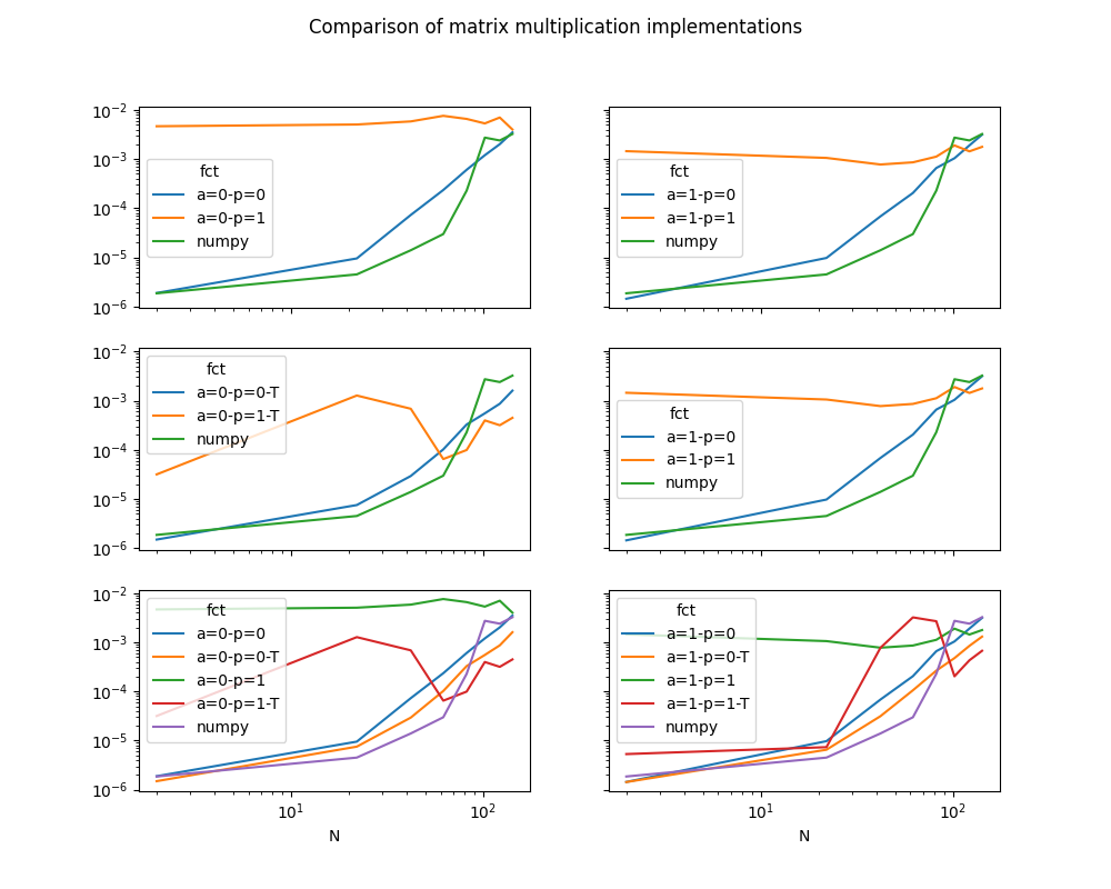
Text(0.5, 0.98, 'Comparison of matrix multiplication implementations')
The results depends on the machine, its number of cores, the compilation settings of numpy or this module.
Total running time of the script: (0 minutes 19.817 seconds)