Note
Go to the end to download the full example code.
Compares filtering implementations (numpy, cython)
The benchmark looks into different ways to implement
thresholding: every value of a vector superior to mx
is replaced by mx (numpy.clip()).
It compares several implementation to numpy.
import pprint
import numpy
import matplotlib.pyplot as plt
from pandas import DataFrame
from teachcompute.validation.cython.experiment_cython import (
    pyfilter_dmax,
    filter_dmax_cython,
    filter_dmax_cython_optim,
    cyfilter_dmax,
    cfilter_dmax,
    cfilter_dmax2,
    cfilter_dmax16,
    cfilter_dmax4,
)
from teachcompute.ext_test_case import measure_time_dim


def get_vectors(fct, n, h=200, dtype=numpy.float64):
    ctxs = [
        dict(
            va=numpy.random.randn(n).astype(dtype),
            fil=fct,
            mx=numpy.float64(0),
            x_name=n,
        )
        for n in range(10, n, h)
    ]
    return ctxs


def numpy_filter(va, mx):
    va[va > mx] = mx


all_res = []
for fct in [
    numpy_filter,
    pyfilter_dmax,
    filter_dmax_cython,
    filter_dmax_cython_optim,
    cyfilter_dmax,
    cfilter_dmax,
    cfilter_dmax2,
    cfilter_dmax16,
    cfilter_dmax4,
]:
    print(fct)
    ctxs = get_vectors(fct, 1000 if fct == pyfilter_dmax else 40000)
    res = list(measure_time_dim("fil(va, mx)", ctxs, verbose=1))
    for r in res:
        r["fct"] = fct.__name__
    all_res.extend(res)

pprint.pprint(all_res[:2])
<function numpy_filter at 0x73e546f874c0>

  0%|          | 0/200 [00:00<?, ?it/s]
 24%|██▍       | 48/200 [00:00<00:00, 474.44it/s]
 48%|████▊     | 96/200 [00:00<00:00, 376.71it/s]
 68%|██████▊   | 135/200 [00:00<00:00, 300.46it/s]
 84%|████████▎ | 167/200 [00:00<00:00, 265.20it/s]
 98%|█████████▊| 195/200 [00:00<00:00, 239.52it/s]
100%|██████████| 200/200 [00:00<00:00, 270.36it/s]
<cyfunction pyfilter_dmax at 0x73e55c97d480>

  0%|          | 0/5 [00:00<?, ?it/s]
100%|██████████| 5/5 [00:00<00:00, 50.01it/s]
<cyfunction filter_dmax_cython at 0x73e54c34e680>

  0%|          | 0/200 [00:00<?, ?it/s]
 42%|████▏     | 83/200 [00:00<00:00, 816.87it/s]
 82%|████████▎ | 165/200 [00:00<00:00, 449.33it/s]
100%|██████████| 200/200 [00:00<00:00, 412.31it/s]
<cyfunction filter_dmax_cython_optim at 0x73e54c34e740>

  0%|          | 0/200 [00:00<?, ?it/s]
 38%|███▊      | 76/200 [00:00<00:00, 748.89it/s]
 76%|███████▌  | 151/200 [00:00<00:00, 490.24it/s]
100%|██████████| 200/200 [00:00<00:00, 418.58it/s]
<cyfunction cyfilter_dmax at 0x73e54c34d480>

  0%|          | 0/200 [00:00<?, ?it/s]
 39%|███▉      | 78/200 [00:00<00:00, 766.25it/s]
 78%|███████▊  | 155/200 [00:00<00:00, 467.88it/s]
100%|██████████| 200/200 [00:00<00:00, 417.68it/s]
<cyfunction cfilter_dmax at 0x73e54c34e8c0>

  0%|          | 0/200 [00:00<?, ?it/s]
 38%|███▊      | 77/200 [00:00<00:00, 762.98it/s]
 77%|███████▋  | 154/200 [00:00<00:00, 351.03it/s]
100%|██████████| 200/200 [00:00<00:00, 328.62it/s]
<cyfunction cfilter_dmax2 at 0x73e54c34e5c0>

  0%|          | 0/200 [00:00<?, ?it/s]
 37%|███▋      | 74/200 [00:00<00:00, 735.42it/s]
 74%|███████▍  | 148/200 [00:00<00:00, 417.50it/s]
 99%|█████████▉| 198/200 [00:00<00:00, 331.38it/s]
100%|██████████| 200/200 [00:00<00:00, 365.40it/s]
<cyfunction cfilter_dmax16 at 0x73e54c34e200>

  0%|          | 0/200 [00:00<?, ?it/s]
 30%|██▉       | 59/200 [00:00<00:00, 574.44it/s]
 58%|█████▊    | 117/200 [00:00<00:00, 311.98it/s]
 78%|███████▊  | 155/200 [00:00<00:00, 235.35it/s]
 92%|█████████▏| 183/200 [00:00<00:00, 186.73it/s]
100%|██████████| 200/200 [00:00<00:00, 207.89it/s]
<cyfunction cfilter_dmax4 at 0x73e547a9dfc0>

  0%|          | 0/200 [00:00<?, ?it/s]
 22%|██▏       | 44/200 [00:00<00:00, 422.21it/s]
 44%|████▎     | 87/200 [00:00<00:00, 224.98it/s]
 57%|█████▊    | 115/200 [00:00<00:00, 159.98it/s]
 68%|██████▊   | 135/200 [00:00<00:00, 132.27it/s]
 76%|███████▌  | 151/200 [00:01<00:00, 116.86it/s]
 82%|████████▏ | 164/200 [00:01<00:00, 102.38it/s]
 88%|████████▊ | 175/200 [00:01<00:00, 93.63it/s]
 92%|█████████▎| 185/200 [00:01<00:00, 86.25it/s]
 97%|█████████▋| 194/200 [00:01<00:00, 78.98it/s]
100%|██████████| 200/200 [00:01<00:00, 111.96it/s]
[{'average': np.float64(1.7740239964041394e-06),
  'context_size': 184,
  'deviation': np.float64(1.5909980042013496e-07),
  'fct': 'numpy_filter',
  'max_exec': np.float64(2.2369999715010635e-06),
  'min_exec': np.float64(1.6720799976610578e-06),
  'number': 50,
  'repeat': 10,
  'ttime': np.float64(1.7740239964041394e-05),
  'warmup_time': 4.341300154919736e-05,
  'x_name': 10},
 {'average': np.float64(1.8300799893040677e-06),
  'context_size': 184,
  'deviation': np.float64(1.1926026711629367e-07),
  'fct': 'numpy_filter',
  'max_exec': np.float64(2.182399985031225e-06),
  'min_exec': np.float64(1.7668199870968239e-06),
  'number': 50,
  'repeat': 10,
  'ttime': np.float64(1.8300799893040677e-05),
  'warmup_time': 1.8763001207844354e-05,
  'x_name': 210}]
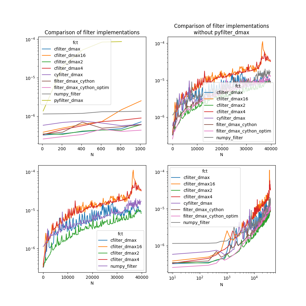
Let’s display the results
cc = DataFrame(all_res)
cc["N"] = cc["x_name"]

fig, ax = plt.subplots(2, 2, figsize=(10, 10))
cc[cc.N <= 1100].pivot(index="N", columns="fct", values="average").plot(
    logy=True, ax=ax[0, 0]
)
cc[cc.fct != "pyfilter_dmax"].pivot(index="N", columns="fct", values="average").plot(
    logy=True, ax=ax[0, 1]
)
cc[cc.fct != "pyfilter_dmax"].pivot(index="N", columns="fct", values="average").plot(
    logy=True, logx=True, ax=ax[1, 1]
)
cc[(cc.fct.str.contains("cfilter") | cc.fct.str.contains("numpy"))].pivot(
    index="N", columns="fct", values="average"
).plot(logy=True, ax=ax[1, 0])
ax[0, 0].set_title("Comparison of filter implementations")
ax[0, 1].set_title("Comparison of filter implementations\nwithout pyfilter_dmax")
Text(0.5, 1.0, 'Comparison of filter implementations\nwithout pyfilter_dmax')
The results depends on the machine, its number of cores, the compilation settings of numpy or this module.
Total running time of the script: (0 minutes 7.904 seconds)