Associativity and matrix multiplication

The matrix multiplication m1 @ m2 @ m3 can be done in two different ways: (m1 @ m2) @ m3 or m1 @ (m2 @ m3). Are these two orders equivalent or is there a better order?

import pprint
import numpy
import matplotlib.pyplot as plt
from pandas import DataFrame
from tqdm import tqdm
from teachcompute.ext_test_case import measure_time

First try

m1 = numpy.random.rand(100, 100)
m2 = numpy.random.rand(100, 10)
m3 = numpy.random.rand(10, 100)

m = m1 @ m2 @ m3

print(m.shape)

mm1 = (m1 @ m2) @ m3
mm2 = m1 @ (m2 @ m3)

print(mm1.shape, mm2.shape)

t1 = measure_time(lambda: (m1 @ m2) @ m3, context={}, number=50, repeat=50)
pprint.pprint(t1)

t2 = measure_time(lambda: m1 @ (m2 @ m3), context={}, number=50, repeat=50)
pprint.pprint(t2)

(100, 100)
(100, 100) (100, 100)
{'average': np.float64(2.515817200019228e-05),
 'context_size': 64,
 'deviation': np.float64(1.0374499508539192e-05),
 'max_exec': np.float64(6.011991999912425e-05),
 'min_exec': np.float64(1.861647999703564e-05),
 'number': 50,
 'repeat': 50,
 'ttime': np.float64(0.001257908600009614),
 'warmup_time': 6.163200009723369e-05}
{'average': np.float64(4.436903639980301e-05),
 'context_size': 64,
 'deviation': np.float64(2.7618504378496756e-06),
 'max_exec': np.float64(6.0102739998910694e-05),
 'min_exec': np.float64(4.262303999894357e-05),
 'number': 50,
 'repeat': 50,
 'ttime': np.float64(0.00221845181999015),
 'warmup_time': 7.618800009367988e-05}

With different sizes

obs = []
for i in tqdm([50, 100, 125, 150, 175, 200]):
    m1 = numpy.random.rand(i, i)
    m2 = numpy.random.rand(i, 10)
    m3 = numpy.random.rand(10, i)

    t1 = measure_time(
        lambda m1=m1, m2=m2, m3=m3: (m1 @ m2) @ m3, context={}, number=50, repeat=50
    )
    t1["formula"] = "(m1 @ m2) @ m3"
    t1["size"] = i
    obs.append(t1)
    t2 = measure_time(
        lambda m1=m1, m2=m2, m3=m3: m1 @ (m2 @ m3), context={}, number=50, repeat=50
    )
    t2["formula"] = "m1 @ (m2 @ m3)"
    t2["size"] = i
    obs.append(t2)

df = DataFrame(obs)
piv = df.pivot(index="size", columns="formula", values="average")
piv

  0%|          | 0/6 [00:00<?, ?it/s]
 33%|███▎      | 2/6 [00:00<00:00,  9.44it/s]
 50%|█████     | 3/6 [00:00<00:00,  5.12it/s]
 67%|██████▋   | 4/6 [00:01<00:00,  3.22it/s]
 83%|████████▎ | 5/6 [00:04<00:01,  1.56s/it]
100%|██████████| 6/6 [00:09<00:00,  2.41s/it]
100%|██████████| 6/6 [00:09<00:00,  1.51s/it]

formula	(m1 @ m2) @ m3	m1 @ (m2 @ m3)
size
50	0.000007	0.000013
100	0.000019	0.000045
125	0.000029	0.000096
150	0.000048	0.000151
175	0.000054	0.001508
200	0.000079	0.001558

Graph

fig, ax = plt.subplots(1, 2, figsize=(12, 4))
piv.plot(
    logx=True,
    logy=True,
    ax=ax[0],
    title=f"{m1.shape!r} @ {m2.shape!r} @ {m3.shape!r}".replace("200", "size"),
)
piv["ratio"] = piv["m1 @ (m2 @ m3)"] / piv["(m1 @ m2) @ m3"]
piv[["ratio"]].plot(ax=ax[1])

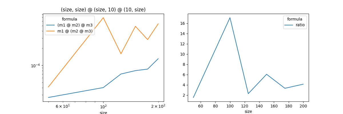
<Axes: xlabel='size'>