Note
Go to the end to download the full example code.
Transformed Target
TransformedTargetRegressor proposes a way to modify the target before training. The notebook extends the concept to classifiers.
TransformedTargetRegressor
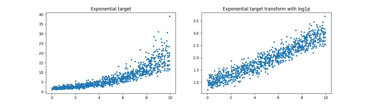
Let’s reuse the example from Effect of transforming the targets in regression model.
import pickle
from pickle import PicklingError
import numpy
from numpy.random import randn, random
from pandas import DataFrame
import matplotlib.pyplot as plt
from sklearn.compose import TransformedTargetRegressor
from sklearn.metrics import accuracy_score, r2_score
from sklearn.linear_model import LinearRegression, LogisticRegression
from sklearn.datasets import load_iris
from sklearn.model_selection import train_test_split
from sklearn.exceptions import ConvergenceWarning
from sklearn.utils._testing import ignore_warnings
from mlinsights.mlmodel import TransformedTargetRegressor2
from mlinsights.mlmodel import TransformedTargetClassifier2


rnd = random((1000, 1))
rndn = randn(1000)
X = rnd[:, :1] * 10
y = rnd[:, 0] * 5 + rndn / 2
y = numpy.exp((y + abs(y.min())) / 2)
y_trans = numpy.log1p(y)
Text(0.5, 1.0, 'Exponential target transform with log1p')
reg = LinearRegression()
reg.fit(X, y)
regr_trans = TransformedTargetRegressor(
    regressor=LinearRegression(), func=numpy.log1p, inverse_func=numpy.expm1
)
regr_trans.fit(X, y)
fig, ax = plt.subplots(1, 2, figsize=(14, 4))
ax[0].plot(X[:, 0], y, ".")
ax[0].plot(X[:, 0], reg.predict(X), ".", label="Regular Linear Regression")
ax[0].set_title("LinearRegression")
ax[1].plot(X[:, 0], y, ".")
ax[1].plot(
    X[:, 0], regr_trans.predict(X), ".", label="Linear Regression with modified target"
)
ax[1].set_title("TransformedTargetRegressor")
Text(0.5, 1.0, 'TransformedTargetRegressor')
TransformedTargetRegressor2
# Same thing with *mlinsights*.


regr_trans2 = TransformedTargetRegressor2(
    regressor=LinearRegression(), transformer="log1p"
)
regr_trans2.fit(X, y)
fig, ax = plt.subplots(1, 3, figsize=(14, 4))
ax[0].plot(X[:, 0], y, ".")
ax[0].plot(X[:, 0], reg.predict(X), ".", label="Regular Linear Regression")
ax[0].set_title("LinearRegression")
ax[1].plot(X[:, 0], y, ".")
ax[1].plot(
    X[:, 0], regr_trans.predict(X), ".", label="Linear Regression with modified target"
)
ax[1].set_title("TransformedTargetRegressor")
ax[2].plot(X[:, 0], y, ".")
ax[2].plot(
    X[:, 0], regr_trans2.predict(X), ".", label="Linear Regression with modified target"
)
ax[2].set_title("TransformedTargetRegressor2")
Text(0.5, 1.0, 'TransformedTargetRegressor2')
It works the same way except the user does not have to specify the inverse function.
Why another?
by1 = pickle.dumps(regr_trans)
by2 = pickle.dumps(regr_trans2)
tr1 = pickle.loads(by1)
tr2 = pickle.loads(by2)
numpy.max(numpy.abs(tr1.predict(X) - tr2.predict(X)))
np.float64(0.0)
Well, to be honest, I did not expect numpy functions to be pickable. Lambda functions are not.
regr_trans3 = TransformedTargetRegressor(
    regressor=LinearRegression(),
    func=lambda x: numpy.log1p(x),
    inverse_func=numpy.expm1,
)
regr_trans3.fit(X, y)
try:
    pickle.dumps(regr_trans3)
except PicklingError as e:
    print(e)
Can't pickle <function <lambda> at 0x79fc006dfc40>: attribute lookup <lambda> on __main__ failed
Classifier and classes permutation
One question I get sometimes from my students is: regression or classification?
reg = LinearRegression()
reg.fit(X_train, y_train)
log = LogisticRegression()
log.fit(X_train, y_train)
(0.8752883470101485, 0.8325991189427313)
The accuracy does not work on the regression output as it produces float.
try:
    accuracy_score(y_test, reg.predict(X_test)), accuracy_score(
        y_test, log.predict(X_test)
    )
except ValueError as e:
    print(e)
Classification metrics can't handle a mix of multiclass and continuous targets
Based on that figure, a regression model would be better than a classification model on a problem which is known to be a classification problem. Let’s play a little bit.
@ignore_warnings(category=(ConvergenceWarning,))
def evaluation():
    rnd = []
    perf_reg = []
    perf_clr = []
    for rs in range(200):
        rnd.append(rs)
        X_train, X_test, y_train, y_test = train_test_split(X, y, random_state=rs)
        reg = LinearRegression()
        reg.fit(X_train, y_train)
        log = LogisticRegression()
        log.fit(X_train, y_train)
        perf_reg.append(r2_score(y_test, reg.predict(X_test)))
        perf_clr.append(r2_score(y_test, log.predict(X_test)))
    return rnd, perf_reg, perf_clr


rnd, perf_reg, perf_clr = evaluation()
fig, ax = plt.subplots(1, 1, figsize=(12, 4))
ax.plot(rnd, perf_reg, label="regression")
ax.plot(rnd, perf_clr, label="classification")
ax.set_title("Comparison between regression and classificaton\non the same problem")
Text(0.5, 1.0, 'Comparison between regression and classificaton\non the same problem')
Difficult to say. Knowing the expected value is an integer. Let’s round the prediction made by the regression which is known to be integer.
def float2int(y):
    return numpy.int32(y + 0.5)


fct2float2int = numpy.vectorize(float2int)
@ignore_warnings(category=(ConvergenceWarning,))
def evaluation2():
    rnd = []
    perf_reg = []
    perf_clr = []
    acc_reg = []
    acc_clr = []
    for rs in range(50):
        rnd.append(rs)
        X_train, X_test, y_train, y_test = train_test_split(X, y, random_state=rs)
        reg = LinearRegression()
        reg.fit(X_train, y_train)
        log = LogisticRegression()
        log.fit(X_train, y_train)
        perf_reg.append(r2_score(y_test, float2int(reg.predict(X_test))))
        perf_clr.append(r2_score(y_test, log.predict(X_test)))
        acc_reg.append(accuracy_score(y_test, float2int(reg.predict(X_test))))
        acc_clr.append(accuracy_score(y_test, log.predict(X_test)))
    return (
        numpy.array(rnd),
        numpy.array(perf_reg),
        numpy.array(perf_clr),
        numpy.array(acc_reg),
        numpy.array(acc_clr),
    )


rnd2, perf_reg2, perf_clr2, acc_reg2, acc_clr2 = evaluation2()
fig, ax = plt.subplots(1, 2, figsize=(14, 4))
ax[0].plot(rnd2, perf_reg2, label="regression")
ax[0].plot(rnd2, perf_clr2, label="classification")
ax[0].set_title(
    "Comparison between regression and classificaton\non the same problem with r2_score"
)
ax[1].plot(rnd2, acc_reg2, label="regression")
ax[1].plot(rnd2, acc_clr2, label="classification")
ax[1].set_title(
    "Comparison between regression and classificaton\n"
    "on the same problem with accuracy_score"
)
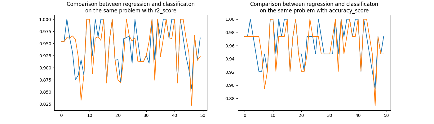
Text(0.5, 1.0, 'Comparison between regression and classificaton\non the same problem with accuracy_score')
Pretty visually indecisive.
numpy.sign(perf_reg2 - perf_clr2).sum()
np.float64(6.0)
numpy.sign(acc_reg2 - acc_clr2).sum()
np.float64(6.0)
As strange as it seems to be, the regression wins on Iris data.
But… There is always a but…
The but…
There is one tiny difference between regression and classification. Classification is immune to a permutation of the label.
reg = LinearRegression()
reg.fit(X_train, y_train)
log = LogisticRegression()
log.fit(X_train, y_train)
(
    r2_score(y_test, fct2float2int(reg.predict(X_test))),
    r2_score(y_test, log.predict(X_test)),
)
(1.0, 0.9609053497942387)
Let’s permute between 1 and 2.
def permute(y):
    y2 = y.copy()
    y2[y == 1] = 2
    y2[y == 2] = 1
    return y2


y_train_permuted = permute(y_train)
y_test_permuted = permute(y_test)
(0.43952802359882015, 0.9626352015732547)
The classifer produces almost the same performance, the regressor seems off. Let’s check that it is just luck.
rows = []
for _i in range(10):
    regpt = TransformedTargetRegressor2(LinearRegression(), transformer="permute")
    regpt.fit(X_train, y_train)
    logpt = TransformedTargetClassifier2(
        LogisticRegression(max_iter=200), transformer="permute"
    )
    logpt.fit(X_train, y_train)
    rows.append(
        {
            "reg_perm": regpt.transformer_.permutation_,
            "reg_score": r2_score(y_test, fct2float2int(regpt.predict(X_test))),
            "log_perm": logpt.transformer_.permutation_,
            "log_score": r2_score(y_test, logpt.predict(X_test)),
        }
    )

df = DataFrame(rows)
df
The classifier produces a constant performance, the regressor is not.
Total running time of the script: (0 minutes 5.192 seconds)