Note
Go to the end to download the full example code.
Piecewise classification with scikit-learn predictors
Piecewise regression is easier to understand but the concept can be extended to classification. That’s what this notebook explores.
Iris dataset and first logistic regression
import matplotlib.pyplot as plt
import seaborn
import numpy
import pandas
from sklearn import datasets
from sklearn.model_selection import train_test_split
from sklearn.linear_model import LogisticRegression
from sklearn.dummy import DummyClassifier
from sklearn.preprocessing import KBinsDiscretizer
from sklearn.metrics import auc, roc_curve
from mlinsights.mlmodel import PiecewiseClassifier

iris = datasets.load_iris()
X = iris.data[:, :2]  # we only take the first two features.
Y = iris.target
X_train, X_test, y_train, y_test = train_test_split(X, Y)
def graph(X, Y, model):
    x_min, x_max = X[:, 0].min() - 0.5, X[:, 0].max() + 0.5
    y_min, y_max = X[:, 1].min() - 0.5, X[:, 1].max() + 0.5
    h = 0.02  # step size in the mesh
    xx, yy = numpy.meshgrid(
        numpy.arange(x_min, x_max, h), numpy.arange(y_min, y_max, h)
    )
    Z = model.predict(numpy.c_[xx.ravel(), yy.ravel()])
    Z = Z.reshape(xx.shape)

    # Put the result into a color plot
    _fig, ax = plt.subplots(1, 1, figsize=(4, 3))
    ax.pcolormesh(xx, yy, Z, cmap=plt.cm.Paired)

    # Plot also the training points
    ax.scatter(X[:, 0], X[:, 1], c=Y, edgecolors="k", cmap=plt.cm.Paired)
    ax.set_xlabel("Sepal length")
    ax.set_ylabel("Sepal width")

    ax.set_xlim(xx.min(), xx.max())
    ax.set_ylim(yy.min(), yy.max())
    ax.set_xticks(())
    ax.set_yticks(())
    return ax


logreg = LogisticRegression()
logreg.fit(X_train, y_train)
ax = graph(X_test, y_test, logreg)
ax.set_title("LogisticRegression")
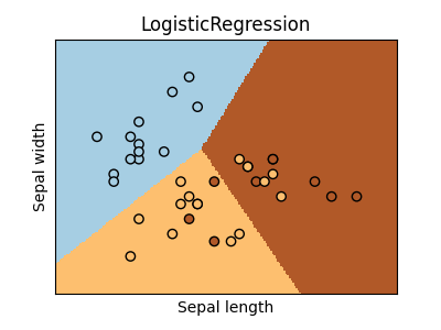
Text(0.5, 1.0, 'LogisticRegression')
Piecewise classication
dummy = DummyClassifier(strategy="most_frequent")
piece4 = PiecewiseClassifier(KBinsDiscretizer(n_bins=2), estimator=dummy, verbose=True)
piece4.fit(X_train, y_train)
~/vv/this312/lib/python3.12/site-packages/sklearn/preprocessing/_discretization.py:296: FutureWarning: The current default behavior, quantile_method='linear', will be changed to quantile_method='averaged_inverted_cdf' in scikit-learn version 1.9 to naturally support sample weight equivalence properties by default. Pass quantile_method='averaged_inverted_cdf' explicitly to silence this warning.
  warnings.warn(
[Parallel(n_jobs=1)]: Done   4 out of   4 | elapsed:    0.0s finished
We look into the bucket given to each point.
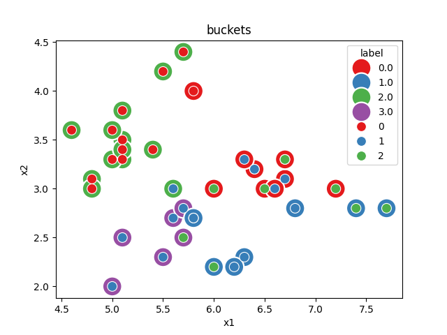
Text(0.5, 1.0, 'buckets')
We see there are four buckets. Two buckets only contains one label. The dummy classifier maps every bucket to the most frequent class in the bucket.
ax = graph(X_test, y_test, piece4)
ax.set_title("Piecewise Classification\n4 buckets")
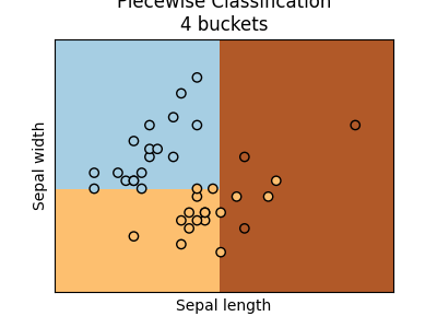
Text(0.5, 1.0, 'Piecewise Classification\n4 buckets')
We can increase the number of buckets.
dummy = DummyClassifier(strategy="most_frequent")
piece9 = PiecewiseClassifier(KBinsDiscretizer(n_bins=3), estimator=dummy, verbose=True)
piece9.fit(X_train, y_train)
~/vv/this312/lib/python3.12/site-packages/sklearn/preprocessing/_discretization.py:296: FutureWarning: The current default behavior, quantile_method='linear', will be changed to quantile_method='averaged_inverted_cdf' in scikit-learn version 1.9 to naturally support sample weight equivalence properties by default. Pass quantile_method='averaged_inverted_cdf' explicitly to silence this warning.
  warnings.warn(
[Parallel(n_jobs=1)]: Done   9 out of   9 | elapsed:    0.0s finished
ax = graph(X_test, y_test, piece9)
ax.set_title("Piecewise Classification\n9 buckets")
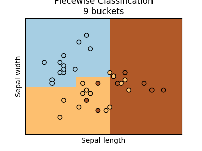
Text(0.5, 1.0, 'Piecewise Classification\n9 buckets')
Let’s compute the ROC curve.
def plot_roc_curve(models, X, y):
    if not isinstance(models, dict):
        return plot_roc_curve({models.__class__.__name__: models}, X, y)

    ax = None
    colors = "bgrcmyk"
    for ic, (name, model) in enumerate(models.items()):
        fpr, tpr, roc_auc = dict(), dict(), dict()
        nb = len(model.classes_)
        y_score = model.predict_proba(X)
        for i in range(nb):
            c = model.classes_[i]
            fpr[i], tpr[i], _ = roc_curve(y_test == c, y_score[:, i])
            roc_auc[i] = auc(fpr[i], tpr[i])

        if ax is None:
            lw = 2
            _, ax = plt.subplots(1, nb, figsize=(4 * nb, 4))
            for i in range(nb):
                ax[i].plot([0, 1], [0, 1], color="navy", lw=lw, linestyle="--")
        plotname = "".join(c for c in name if "A" <= c <= "Z" or "0" <= c <= "9")
        for i in range(nb):
            ax[i].plot(
                fpr[i],
                tpr[i],
                color=colors[ic],
                lw=lw,
                label="%0.2f %s" % (roc_auc[i], plotname),
            )
            ax[i].set_title("class {}".format(model.classes_[i]))
    for k in range(ax.shape[0]):
        ax[k].legend()
    return ax


plot_roc_curve({"LR": logreg, "P4": piece4, "P9": piece9}, X_test, y_test)
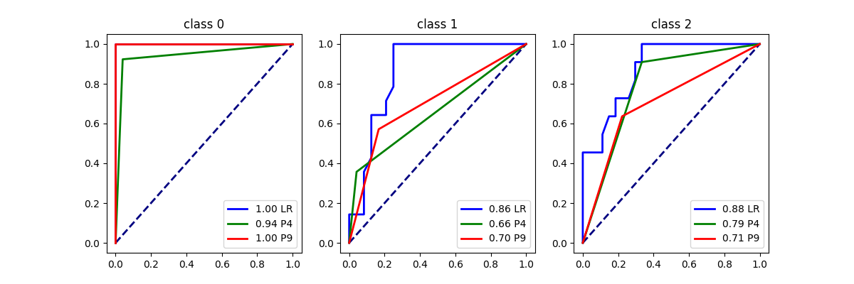
array([<Axes: title={'center': 'class 0'}>,
       <Axes: title={'center': 'class 1'}>,
       <Axes: title={'center': 'class 2'}>], dtype=object)
Let’s use the decision tree to create buckets.
dummy = DummyClassifier(strategy="most_frequent")
pieceT = PiecewiseClassifier("tree", estimator=dummy, verbose=True)
pieceT.fit(X_train, y_train)
[Parallel(n_jobs=1)]: Done 14 out of 14 | elapsed: 0.0s finished
ax = graph(X_test, y_test, pieceT)
ax.set_title("Piecewise Classification\n%d buckets (tree)" % len(pieceT.estimators_))
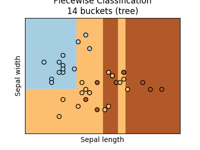
Text(0.5, 1.0, 'Piecewise Classification\n14 buckets (tree)')
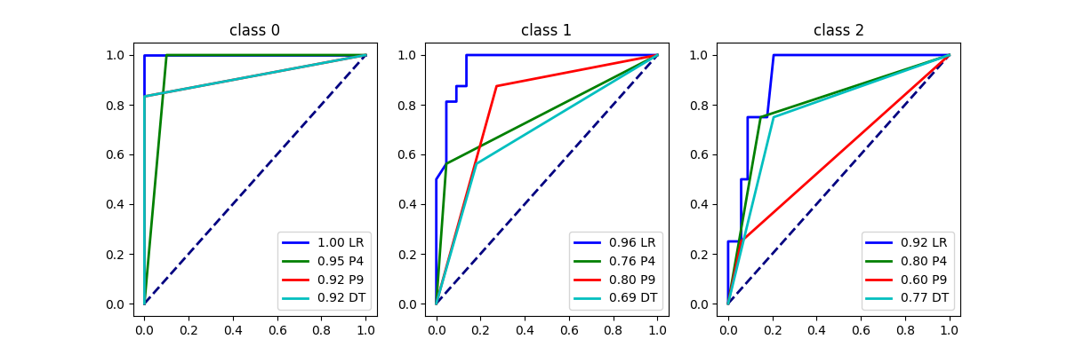
array([<Axes: title={'center': 'class 0'}>,
       <Axes: title={'center': 'class 1'}>,
       <Axes: title={'center': 'class 2'}>], dtype=object)
Total running time of the script: (0 minutes 2.904 seconds)