Quantile Regression

scikit-learn does not have a quantile regression. mlinsights implements a version of it.

Simple example

We first generate some dummy data.

import numpy
import matplotlib.pyplot as plt
from pandas import DataFrame
from sklearn.linear_model import LinearRegression
from mlinsights.mlmodel import QuantileLinearRegression

X = numpy.random.random(1000)
eps1 = (numpy.random.random(900) - 0.5) * 0.1
eps2 = (numpy.random.random(100)) * 10
eps = numpy.hstack([eps1, eps2])
X = X.reshape((1000, 1))
Y = X.ravel() * 3.4 + 5.6 + eps

clr = LinearRegression()
clr.fit(X, Y)

LinearRegression()

In a Jupyter environment, please rerun this cell to show the HTML representation or trust the notebook.
On GitHub, the HTML representation is unable to render, please try loading this page with nbviewer.org.

clq = QuantileLinearRegression()
clq.fit(X, Y)


data = dict(X=X.ravel(), Y=Y, clr=clr.predict(X), clq=clq.predict(X))
df = DataFrame(data)
df.head()

	X	Y	clr	clq
0	0.253591	6.451220	6.873732	6.474578
1	0.273386	6.530336	6.946194	6.541909
2	0.981536	8.901532	9.538408	8.950581
3	0.189410	6.240350	6.638796	6.256276
4	0.008886	5.591083	5.977979	5.642248

fig, ax = plt.subplots(1, 1, figsize=(10, 4))
choice = numpy.random.choice(X.shape[0] - 1, size=100)
xx = X.ravel()[choice]
yy = Y[choice]
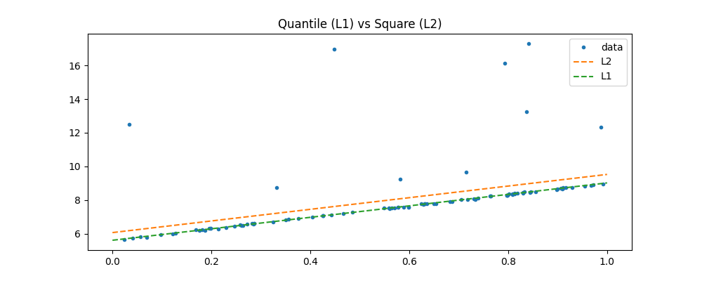
ax.plot(xx, yy, ".", label="data")
xx = numpy.array([[0], [1]])
y1 = clr.predict(xx)
y2 = clq.predict(xx)
ax.plot(xx, y1, "--", label="L2")
ax.plot(xx, y2, "--", label="L1")
ax.set_title("Quantile (L1) vs Square (L2)")
ax.legend()

<matplotlib.legend.Legend object at 0x7dd1aac05b80>

The L1 is clearly less sensible to extremas. The optimization algorithm is based on Iteratively reweighted least squares. It estimates a linear regression with error L2 then reweights each oberservation with the inverse of the error L1.

clq = QuantileLinearRegression(verbose=True, max_iter=20)
clq.fit(X, Y)

[QuantileLinearRegression.fit] iter=1 error=853.9008145418201
[QuantileLinearRegression.fit] iter=2 error=546.3665130625367
[QuantileLinearRegression.fit] iter=3 error=496.098333075342
[QuantileLinearRegression.fit] iter=4 error=495.7617127189459
[QuantileLinearRegression.fit] iter=5 error=495.4216843950596
[QuantileLinearRegression.fit] iter=6 error=495.20197898886244
[QuantileLinearRegression.fit] iter=7 error=495.0334627319531
[QuantileLinearRegression.fit] iter=8 error=494.92642428728277
[QuantileLinearRegression.fit] iter=9 error=494.82861984158745
[QuantileLinearRegression.fit] iter=10 error=494.76065181513496
[QuantileLinearRegression.fit] iter=11 error=494.71516121613246
[QuantileLinearRegression.fit] iter=12 error=494.6744424392276
[QuantileLinearRegression.fit] iter=13 error=494.6463271066102
[QuantileLinearRegression.fit] iter=14 error=494.6180033247077
[QuantileLinearRegression.fit] iter=15 error=494.59973985026437
[QuantileLinearRegression.fit] iter=16 error=494.58365013787017
[QuantileLinearRegression.fit] iter=17 error=494.56462829562474
[QuantileLinearRegression.fit] iter=18 error=494.54836863328563
[QuantileLinearRegression.fit] iter=19 error=494.53616162309544
[QuantileLinearRegression.fit] iter=20 error=494.5273731709936

QuantileLinearRegression(max_iter=20, verbose=True)

In a Jupyter environment, please rerun this cell to show the HTML representation or trust the notebook.
On GitHub, the HTML representation is unable to render, please try loading this page with nbviewer.org.

clq.score(X, Y)

0.4945273731709936

Regression with various quantiles

X = numpy.random.random(1200)
eps1 = (numpy.random.random(900) - 0.5) * 0.5
eps2 = (numpy.random.random(300)) * 2
eps = numpy.hstack([eps1, eps2])
X = X.reshape((1200, 1))
Y = X.ravel() * 3.4 + 5.6 + eps + X.ravel() * X.ravel() * 8

fig, ax = plt.subplots(1, 1, figsize=(10, 4))
choice = numpy.random.choice(X.shape[0] - 1, size=100)
xx = X.ravel()[choice]
yy = Y[choice]
ax.plot(xx, yy, ".", label="data")
ax.set_title("Almost linear dataset")

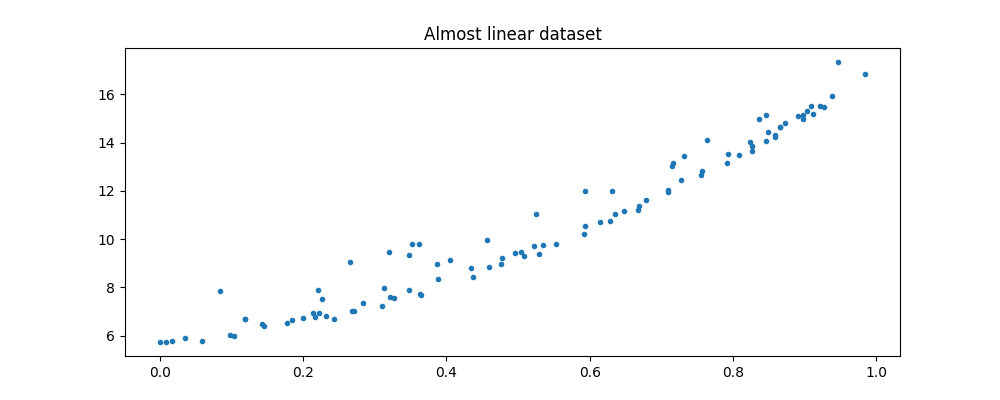
Text(0.5, 1.0, 'Almost linear dataset')

clqs = {}
for qu in [0.1, 0.25, 0.5, 0.75, 0.9]:
    clq = QuantileLinearRegression(quantile=qu)
    clq.fit(X, Y)
    clqs["q=%1.2f" % qu] = clq

fig, ax = plt.subplots(1, 1, figsize=(10, 4))
choice = numpy.random.choice(X.shape[0] - 1, size=100)
xx = X.ravel()[choice]
yy = Y[choice]
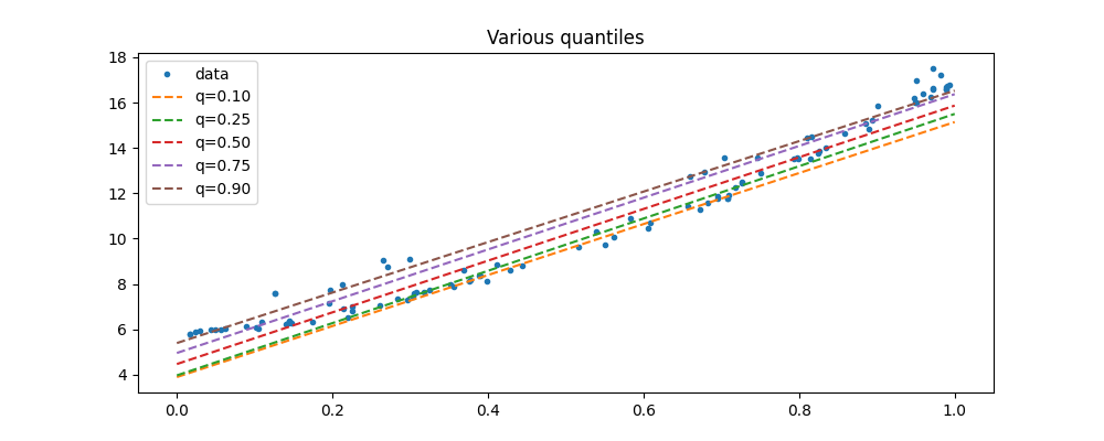
ax.plot(xx, yy, ".", label="data")
xx = numpy.array([[0], [1]])
for qu in sorted(clqs):
    y = clqs[qu].predict(xx)
    ax.plot(xx, y, "--", label=qu)
ax.set_title("Various quantiles")
ax.legend()

<matplotlib.legend.Legend object at 0x7dd1acd379b0>