Regression with confidence interval

The notebook computes confidence intervals with bootstrapping and quantile regression on a simple problem.

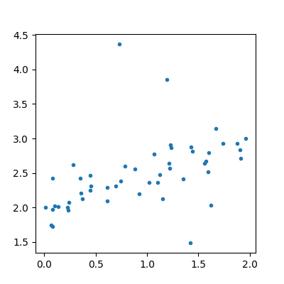
Some data

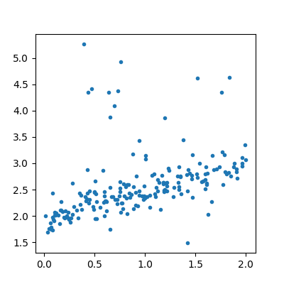
The data follows the formula: . Noises follows the laws , , . The second part of the noise adds some bigger noise but not always.

import numpy
from numpy.random import binomial, rand, randn
import pandas
import matplotlib.pyplot as plt
import seaborn as sns
from sklearn.model_selection import train_test_split
from sklearn.gaussian_process import GaussianProcessRegressor
from sklearn.gaussian_process.kernels import (
    RBF,
    ConstantKernel as C,
    WhiteKernel,
)
from sklearn.linear_model import LinearRegression
from sklearn.tree import DecisionTreeRegressor
from mlinsights.mlmodel import IntervalRegressor, QuantileLinearRegression


N = 200
X = rand(N, 1) * 2
eps = randn(N, 1) * 0.2
eps2 = randn(N, 1) + 1
bin = binomial(2, 0.05, size=(N, 1))
y = (0.5 * X + eps + 2 + eps2 * bin).ravel()

fig, ax = plt.subplots(1, 1, figsize=(4, 4))
ax.plot(X, y, ".")

[<matplotlib.lines.Line2D object at 0x7dd2191cbe60>]

X_train, X_test, y_train, y_test = train_test_split(X, y)

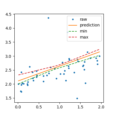
Confidence interval with a linear regression

# The object fits many times the same learner, every training is done on a
# resampling of the training dataset.


lin = IntervalRegressor(LinearRegression())
lin.fit(X_train, y_train)

IntervalRegressor(estimator=LinearRegression())

In a Jupyter environment, please rerun this cell to show the HTML representation or trust the notebook.
On GitHub, the HTML representation is unable to render, please try loading this page with nbviewer.org.

sorted_X = numpy.array(list(sorted(X_test)))
pred = lin.predict(sorted_X)
bootstrapped_pred = lin.predict_sorted(sorted_X)
min_pred = bootstrapped_pred[:, 0]
max_pred = bootstrapped_pred[:, bootstrapped_pred.shape[1] - 1]

fig, ax = plt.subplots(1, 1, figsize=(4, 4))
ax.plot(X_test, y_test, ".", label="raw")
ax.plot(sorted_X, pred, label="prediction")
ax.plot(sorted_X, min_pred, "--", label="min")
ax.plot(sorted_X, max_pred, "--", label="max")
ax.legend()

<matplotlib.legend.Legend object at 0x7dd2124e1cd0>

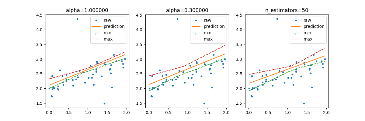
Higher confidence interval

# It is possible to use smaller resample of the training dataset or we can
# increase the number of resamplings.


lin2 = IntervalRegressor(LinearRegression(), alpha=0.3)
lin2.fit(X_train, y_train)

IntervalRegressor(alpha=0.3, estimator=LinearRegression())

In a Jupyter environment, please rerun this cell to show the HTML representation or trust the notebook.
On GitHub, the HTML representation is unable to render, please try loading this page with nbviewer.org.

lin3 = IntervalRegressor(LinearRegression(), n_estimators=50)
lin3.fit(X_train, y_train)

IntervalRegressor(estimator=LinearRegression(), n_estimators=50)

In a Jupyter environment, please rerun this cell to show the HTML representation or trust the notebook.
On GitHub, the HTML representation is unable to render, please try loading this page with nbviewer.org.

pred2 = lin2.predict(sorted_X)
bootstrapped_pred2 = lin2.predict_sorted(sorted_X)
min_pred2 = bootstrapped_pred2[:, 0]
max_pred2 = bootstrapped_pred2[:, bootstrapped_pred2.shape[1] - 1]

pred3 = lin3.predict(sorted_X)
bootstrapped_pred3 = lin3.predict_sorted(sorted_X)
min_pred3 = bootstrapped_pred3[:, 0]
max_pred3 = bootstrapped_pred3[:, bootstrapped_pred3.shape[1] - 1]

fig, ax = plt.subplots(1, 3, figsize=(12, 4))
ax[0].plot(X_test, y_test, ".", label="raw")
ax[0].plot(sorted_X, pred, label="prediction")
ax[0].plot(sorted_X, min_pred, "--", label="min")
ax[0].plot(sorted_X, max_pred, "--", label="max")
ax[0].legend()
ax[0].set_title("alpha=%f" % lin.alpha)
ax[1].plot(X_test, y_test, ".", label="raw")
ax[1].plot(sorted_X, pred2, label="prediction")
ax[1].plot(sorted_X, min_pred2, "--", label="min")
ax[1].plot(sorted_X, max_pred2, "--", label="max")
ax[1].set_title("alpha=%f" % lin2.alpha)
ax[1].legend()
ax[2].plot(X_test, y_test, ".", label="raw")
ax[2].plot(sorted_X, pred3, label="prediction")
ax[2].plot(sorted_X, min_pred3, "--", label="min")
ax[2].plot(sorted_X, max_pred3, "--", label="max")
ax[2].set_title("n_estimators=%d" % lin3.n_estimators)
ax[2].legend()

<matplotlib.legend.Legend object at 0x7dd2192a0ef0>

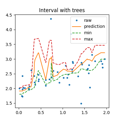
With decision trees

tree = IntervalRegressor(DecisionTreeRegressor(min_samples_leaf=10))
tree.fit(X_train, y_train)

IntervalRegressor(estimator=DecisionTreeRegressor(min_samples_leaf=10))

In a Jupyter environment, please rerun this cell to show the HTML representation or trust the notebook.
On GitHub, the HTML representation is unable to render, please try loading this page with nbviewer.org.

pred_tree = tree.predict(sorted_X)
b_pred_tree = tree.predict_sorted(sorted_X)
min_pred_tree = b_pred_tree[:, 0]
max_pred_tree = b_pred_tree[:, b_pred_tree.shape[1] - 1]

fig, ax = plt.subplots(1, 1, figsize=(4, 4))
ax.plot(X_test, y_test, ".", label="raw")
ax.plot(sorted_X, pred_tree, label="prediction")
ax.plot(sorted_X, min_pred_tree, "--", label="min")
ax.plot(sorted_X, max_pred_tree, "--", label="max")
ax.set_title("Interval with trees")
ax.legend()

<matplotlib.legend.Legend object at 0x7dd219a8d1c0>

In that case, the prediction is very similar to the one a random forest would produce as it is an average of the predictions made by 10 trees.

Regression quantile

The last way tries to fit two regressions for quantiles 0.05 and 0.95.

m = QuantileLinearRegression()
q1 = QuantileLinearRegression(quantile=0.05)
q2 = QuantileLinearRegression(quantile=0.95)
for model in [m, q1, q2]:
    model.fit(X_train, y_train)

fig, ax = plt.subplots(1, 1, figsize=(4, 4))
ax.plot(X_test, y_test, ".", label="raw")

[<matplotlib.lines.Line2D object at 0x7dd219a68950>]

for label, model in [("med", m), ("q0.05", q1), ("q0.95", q2)]:
    p = model.predict(sorted_X)
    ax.plot(sorted_X, p, label=label)
ax.set_title("Quantile Regression")
ax.legend()

<matplotlib.legend.Legend object at 0x7dd2199ee3f0>

With a non linear model… but the model QuantileMLPRegressor only implements the regression with quantile 0.5.

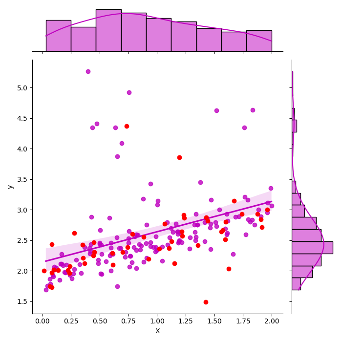
With seaborn

It uses a theoritical way to compute the confidence interval by computing the confidence interval on the parameters first.

df_train = pandas.DataFrame(dict(X=X_train.ravel(), y=y_train))
g = sns.jointplot(x="X", y="y", data=df_train, kind="reg", color="m", height=7)
g.ax_joint.plot(X_test, y_test, "ro")

[<matplotlib.lines.Line2D object at 0x7dd21927ad20>]

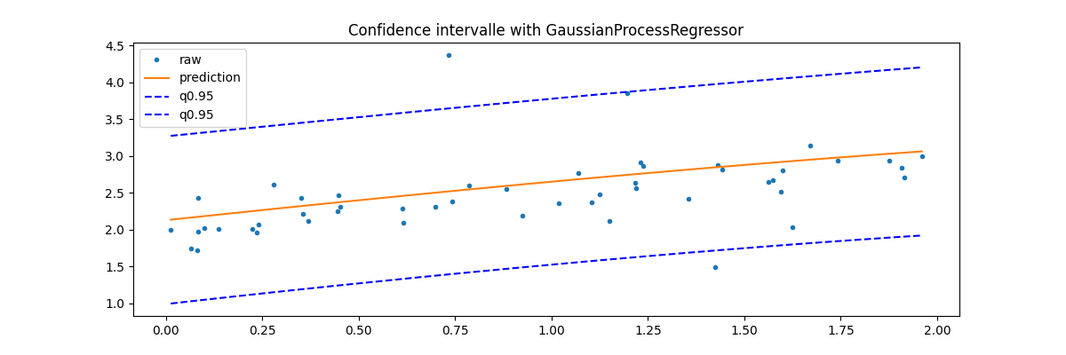
GaussianProcessRegressor

Last option with this example Gaussian Processes regression: basic introductory example which computes the standard deviation for every prediction. It can then be used to show an interval confidence.

kernel = C(1.0, (1e-3, 1e3)) * RBF(10, (1e-2, 1e2)) + WhiteKernel()
gp = GaussianProcessRegressor(kernel=kernel, n_restarts_optimizer=9)
gp.fit(X_train, y_train)

GaussianProcessRegressor(kernel=1**2 * RBF(length_scale=10) + WhiteKernel(noise_level=1),
                         n_restarts_optimizer=9)

In a Jupyter environment, please rerun this cell to show the HTML representation or trust the notebook.
On GitHub, the HTML representation is unable to render, please try loading this page with nbviewer.org.

y_pred, sigma = gp.predict(sorted_X, return_std=True)

fig, ax = plt.subplots(1, 1, figsize=(12, 4))
ax.plot(X_test, y_test, ".", label="raw")
ax.plot(sorted_X, y_pred, label="prediction")
ax.plot(sorted_X, y_pred + sigma * 1.96, "b--", label="q0.95")
ax.plot(sorted_X, y_pred - sigma * 1.96, "b--", label="q0.95")
ax.set_title("Confidence intervalle with GaussianProcessRegressor")
ax.legend()

<matplotlib.legend.Legend object at 0x7dd21917fc80>