numpy.digitize as a tree

Function numpy.digitize() transforms a real variable into a discrete one by returning the buckets the variable falls into. This bucket can be efficiently retrieved by doing a binary search over the bins. That’s equivalent to decision tree. Function digitize2tree.

Simple example

import numpy
import matplotlib.pyplot as plt
from onnxruntime import InferenceSession
from pandas import DataFrame, pivot, pivot_table
from skl2onnx import to_onnx
from sklearn.tree import export_text
from tqdm import tqdm
from mlinsights.ext_test_case import measure_time
from mlinsights.mltree import digitize2tree

x = numpy.array([0.2, 6.4, 3.0, 1.6])
bins = numpy.array([0.0, 1.0, 2.5, 4.0, 7.0])
expected = numpy.digitize(x, bins, right=True)
tree = digitize2tree(bins, right=True)
pred = tree.predict(x.reshape((-1, 1)))
print(expected, pred)

[1 4 3 2] [1. 4. 3. 2.]

The tree looks like the following.

print(export_text(tree, feature_names=["x"]))

|--- x <= 2.50
|   |--- x <= 1.00
|   |   |--- x <= 0.00
|   |   |   |--- value: [0.00]
|   |   |--- x >  0.00
|   |   |   |--- value: [1.00]
|   |--- x >  1.00
|   |   |--- value: [2.00]
|--- x >  2.50
|   |--- x <= 4.00
|   |   |--- x <= 2.50
|   |   |   |--- value: [2.00]
|   |   |--- x >  2.50
|   |   |   |--- value: [3.00]
|   |--- x >  4.00
|   |   |--- x <= 7.00
|   |   |   |--- x <= 4.00
|   |   |   |   |--- value: [3.00]
|   |   |   |--- x >  4.00
|   |   |   |   |--- value: [4.00]
|   |   |--- x >  7.00
|   |   |   |--- value: [5.00]

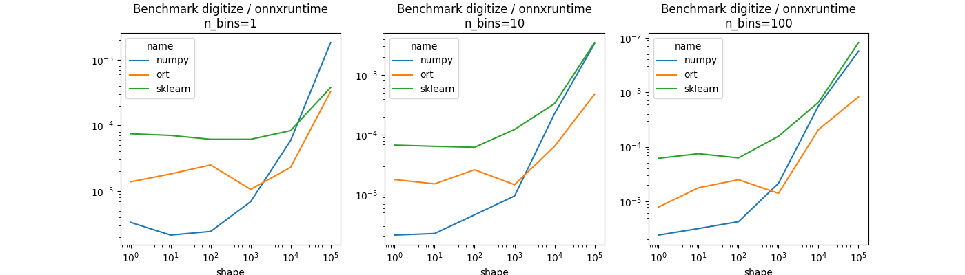
Benchmark

Let’s measure the processing time. numpy should be much faster than scikit-learn as it is adding many verification. However, the benchmark also includes a conversion of the tree into ONNX and measure the processing time with onnxruntime.

obs = []

for shape in tqdm([1, 10, 100, 1000, 10000, 100000]):
    x = numpy.random.random(shape).astype(numpy.float32)
    if shape < 1000:
        repeat = number = 100
    else:
        repeat = number = 10

    for n_bins in [1, 10, 100]:
        bins = (numpy.arange(n_bins) / n_bins).astype(numpy.float32)

        ti = measure_time(
            "numpy.digitize(x, bins, right=True)",
            context={"numpy": numpy, "x": x, "bins": bins},
            div_by_number=True,
            repeat=repeat,
            number=number,
        )
        ti["name"] = "numpy"
        ti["n_bins"] = n_bins
        ti["shape"] = shape
        obs.append(ti)

        tree = digitize2tree(bins, right=True)

        ti = measure_time(
            "tree.predict(x)",
            context={"numpy": numpy, "x": x.reshape((-1, 1)), "tree": tree},
            div_by_number=True,
            repeat=repeat,
            number=number,
        )
        ti["name"] = "sklearn"
        ti["n_bins"] = n_bins
        ti["shape"] = shape
        obs.append(ti)

        onx = to_onnx(tree, x.reshape((-1, 1)), target_opset=15)

        sess = InferenceSession(
            onx.SerializeToString(), providers=["CPUExecutionProvider"]
        )

        ti = measure_time(
            "sess.run(None, {'X': x})",
            context={"numpy": numpy, "x": x.reshape((-1, 1)), "sess": sess},
            div_by_number=True,
            repeat=repeat,
            number=number,
        )
        ti["name"] = "ort"
        ti["n_bins"] = n_bins
        ti["shape"] = shape
        obs.append(ti)


df = DataFrame(obs)
piv = pivot_table(
    data=df, index="shape", columns=["n_bins", "name"], values=["average"]
)
print(piv)

  0%|          | 0/6 [00:00<?, ?it/s]
 17%|█▋        | 1/6 [00:02<00:12,  2.58s/it]
 33%|███▎      | 2/6 [00:05<00:10,  2.66s/it]
 50%|█████     | 3/6 [00:08<00:08,  2.71s/it]
 83%|████████▎ | 5/6 [00:08<00:01,  1.27s/it]
100%|██████████| 6/6 [00:10<00:00,  1.62s/it]
100%|██████████| 6/6 [00:10<00:00,  1.81s/it]
         average
n_bins       1                             10                            100
name       numpy       ort   sklearn     numpy       ort   sklearn     numpy       ort   sklearn
shape
1       0.000003  0.000014  0.000074  0.000002  0.000018  0.000067  0.000002  0.000008  0.000061
10      0.000002  0.000018  0.000070  0.000002  0.000015  0.000064  0.000003  0.000018  0.000075
100     0.000002  0.000025  0.000061  0.000005  0.000026  0.000062  0.000004  0.000025  0.000063
1000    0.000007  0.000011  0.000061  0.000010  0.000015  0.000123  0.000021  0.000014  0.000156
10000   0.000059  0.000023  0.000083  0.000226  0.000064  0.000332  0.000565  0.000206  0.000655
100000  0.001816  0.000327  0.000377  0.003350  0.000478  0.003467  0.005651  0.000823  0.008116

Plotting

n_bins = list(sorted(set(df.n_bins)))
fig, ax = plt.subplots(1, len(n_bins), figsize=(14, 4))

for i, nb in enumerate(n_bins):
    piv = pivot(
        data=df[df.n_bins == nb], index="shape", columns="name", values="average"
    )
    piv.plot(
        title="Benchmark digitize / onnxruntime\nn_bins=%d" % nb,
        logx=True,
        logy=True,
        ax=ax[i],
    )